
Solving Addition Equations Using Scales
Loading the math board and drawing, please wait…
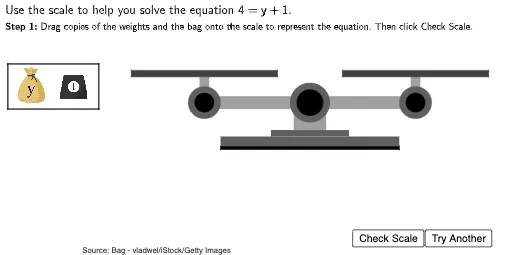
This example demonstrates how to solve addition equations using a dynamic balance scale, visually representing the concept of equilibrium and inverse operations. Core math concepts include equation balancing, addition inverses, and algebraic solutions. Constructed with GeoGebra commands like Polygon, Circle, Random, Frequency, and Textfield, featuring objects such as ScaleBottom1, ScaleArm, and Locus. Ideal for middle school mathematics education to visualize equation-solving processes.
GeoGebra Commands & Parameters
Polygon((2.75, 1.95), (2.75, 2.05), (8.25, 2.05), (8.25, 1.95)) → ScaleBottom1, f, g, h, iPolygon((4.3, 2.35), (4.3, 2.55), (6.7, 2.55), (6.7, 2.35)) → ScaleBottom3, n, p, q, rPolygon((5, 2.55), (5, 3.25), (6, 3.25), (6, 2.55)) → ScaleBottom4, s, t, d, ePolygon((2.75, 2.05), (2.75, 2.35), (8.25, 2.35), (8.25, 2.05)) → ScaleBottom2, j, k, l, mPolygon(Left + (0, 0.2), Left - (0, 0.2), Right - (0, 0.2), Right + (0, 0.2)) → ScaleArm, f_1, g_1, h_1, i_1Circle(Left, 0.5) → LeftArmCircle1Circle(Left, 0.3) → LeftArmCircle2Circle(Right, 0.5) → RightArmCircle1Circle(Right, 0.3) → RightArmCircle2Polygon(Left - (0.15, 0), Left + (0.15, 0), Left + (0.15, 0.8), Left + (-0.15, 0.8)) → LeftArmStand, j_1, k_1, l_1, m_1Polygon(Right - (0.15, 0), Right + (0.15, 0), Right + (0.15, 0.8), Right + (-0.15, 0.8)) → RightArmStand, n_1, p_1, q_1, r_1Polygon(Left + (-2.25, 0.8), Left + (-2.25, 1), Left + (2.25, 1), Left + (2.25, 0.8)) → LeftTray, s_1, t_1, a_1, b_1Polygon(Right + (-2.25, 0.8), Right + (-2.25, 1), Right + (2.25, 1), Right + (2.25, 0.8)) → RightTray, c_1, d_1, e_1, f_2Circle((5.5, 3.4), 0.6) → ScaleBottom5Circle((5.5, 3.4), 0.4) → ScaleBottom6Random(1, 2) → sideorderPolygon((-3.8, 4.6), (-1, 4.6), (-1, 3.2), (-3.8, 3.2)) → ImageBox, c, g_2, h_2, i_2Frequency(Sort[Insert[{0, 1, 2}, Last[ImageLocator, 19], -1]]) → OccurencesTextfield(usertext) → InputBox1