
Slope Field
Loading the math board and drawing, please wait…
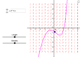
This example demonstrates the slope field of a differential equation, visually showing the distribution of solution curves. Core math concepts include calculus-based slope fields, differential equations, and direction fields. Construction highlights: uses SlopeField for plotting, SolveODE for numerical solutions, Textfield for annotations, and Polygon for shapes. Suitable for high school and above students learning differential equations and numerical methods, or for educational demonstrations.
GeoGebra Commands & Parameters
SlopeField(f, n, a, -5, -5, 5, 5) → slopefield1SolveODE(f, x(A), y(A), 5, 0.05) → numericalIntegral1SolveODE(f, x(A), y(A), -5, 0.05) → numericalIntegral2Textfield(f) → inputBox1Polygon((-100, -100), (-5.7, -100), (-5.7, 100), (-100, 100)) → poly1, b, c, d, e
AI Drawing Prompt Reference
Draw a slope field for a differential equation using colored short arrows to indicate the slope at each grid point, and add several numerical solution curves passing through specified points that align with the direction of the slope field, annotate the equation, and enclose the entire graphic with a rectangular frame.
The prompt above was compiled from the original drawing commands and is for reference only.