
Sketching Graphs from Derivative Information
Loading the math board and drawing, please wait…
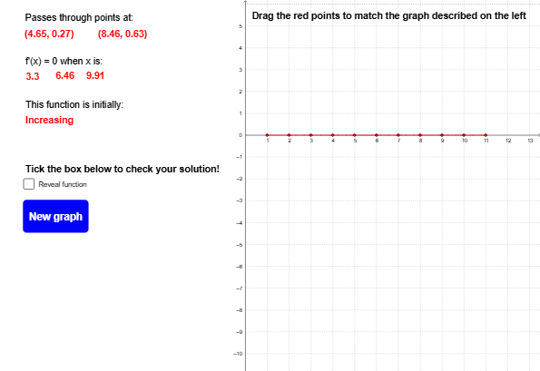
This GeoGebra example demonstrates how to sketch a function's graph based on derivative information, such as extrema and inflection points. It illustrates the relationship between the sign of the derivative, monotonicity, concavity, and the shape of the curve. The construction uses commands like FitPoly to fit polynomial segments, Extremum and TurningPoint to automatically locate critical and inflection points, and Text, If, Segment, Point for annotations and connecting segments. Objects include multiple points (A, B, C, etc.), line segments (segA to segK), and parabolic arcs (parABC, parBCD, etc.) that approximate the function between key points. This is ideal for high school or introductory college calculus students to visualize how derivative information guides graph sketching.
GeoGebra Commands & Parameters
Text("This function is initially:") → text8Text("f'(x) = 0 when x is:") → text4If(f'(1) < 0, "Decreasing", "Increasing") → text9Segment((1, -5), (1, 5)) → segASegment((2, -5), (2, 5)) → segBSegment((3, -5), (3, 5)) → segCSegment((4, -5), (4, 5)) → segDSegment((5, -5), (5, 5)) → segESegment((6, -5), (6, 5)) → segFSegment((7, -5), (7, 5)) → segGSegment((8, -5), (8, 5)) → segHSegment((9, -5), (9, 5)) → segISegment((10, -5), (10, 5)) → segJSegment((11, -5), (11, 5)) → segKPoint(segA) → ZAPoint(segB) → ZBPoint(segC) → ZCPoint(segD) → ZDPoint(segE) → ZEPoint(segF) → ZFPoint(segG) → ZGPoint(segH) → ZHPoint(segI) → ZIPoint(segJ) → ZJPoint(segK) → ZKFitPoly({ZA, ZB, ZC}, 2) → parABCFitPoly({ZB, ZC, ZD}, 2) → parBCDFitPoly({ZC, ZD, ZE}, 2) → parCDEFitPoly({ZD, ZE, ZF}, 2) → parDEFFitPoly({ZE, ZF, ZG}, 2) → parEFGFitPoly({ZF, ZG, ZH}, 2) → parFGHFitPoly({ZG, ZH, ZI}, 2) → parGHIFitPoly({ZH, ZI, ZJ}, 2) → parHIJFitPoly({ZI, ZJ, ZK}, 2) → parIJKText("Tick the box below to check your solution!") → text11Text("Passes through points at:") → text1Text("Drag the red points to match the graph described on the left") → text10FitPoly({A, B, C, D, E}, 4) → pExtremum(p, 1, 11) → TP_1, TP_2, TP_3Text(x(TP_1)) → stattext1TurningPoint(p) → IP_1, IP_2Text(IP_1) → inftext1Text(IP_2) → inftext2Text(x(TP_2)) → stattext2Text(x(TP_3)) → stattext3