
Deriving the Tangent Graph from the Unit Circle
Loading the math board and drawing, please wait…
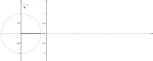
This GeoGebra example dynamically demonstrates how the tangent function (tan θ) graph is derived from the unit circle through geometric construction. It visualizes the relationship between an angle θ rotating on the unit circle and the corresponding tangent value plotted on a coordinate plane. Core mathematical concepts include the unit circle, definitions of sine, cosine, and tangent, angle measurement in radians, and the generation of a function graph. The construction uses GeoGebra commands such as Point, Rotate, Segment, Angle, Circle, Vector, Sequence, and Function to create the circle, rotating radius, angle labels, and a sequence of points that trace the tangent curve. This resource is ideal for high school or introductory college students learning trigonometry, as well as for teachers demonstrating the periodic nature, asymptotes, and geometric origin of the tangent function.
GeoGebra Commands & Parameters
Point(Ray[(0, 0), (-1, 0)]) → BRotate(A, θ, B) → PSegment(A, Intersect[Line[B, P], x = x(A)]) → hSegment(P, Intersect[Line[B, P], x = x(A)]) → gRotate(A, θ, B) → A'Angle(A, B, A') → αRotate(A, θ, B) → A'_1Angle(A, B, A'_1) → βSegment(Q, (x(Q), 0)) → eCircle(B, A) → cSegment(B, P) → aVector((x(B), y(Corner[1])), (x(B), y(Corner[4]))) → uVector((0, y(Corner[1])), (0, y(Corner[4]))) → wVector((0, 0), (x(Corner[2]), 0)) → zSequence(Segment[((0.75 * i), 0), ((0.75 * i), -0.025)], i, 1, 4) → list1Vector(B - (1.2, 0), B + (1.2, 0)) → vSequence(Segment[(0, (0.5 * i) - 1), (-0.025, (0.5 * i) - 1)], i, 0, 4) → list2Sequence(Segment[(x(B), (0.5 * i) - 1), (x(B) - 0.025, (0.5 * i) - 1)], i, 0, 4) → list3Sequence(Segment[B + ((0.5 * i) - 1, 0), B + ((0.5 * i) - 1, -0.025)], i, 0, 4) → list4Segment(C, Q) → dFunction(tan((120° * x)), 0, (θ / ((360 * γ)) * 3)) → fPoint(Ray[(0, 0), (-1, 0)]) → B_1Rotate(A_1, θ, B_1) → P_1Rotate(A_1, θ, B_1) → A'_2Rotate(A_1, θ, B_1) → A'_3Circle(B_1, A_1) → c_1