
Simulation and Normal Distribution
Loading the math board and drawing, please wait…
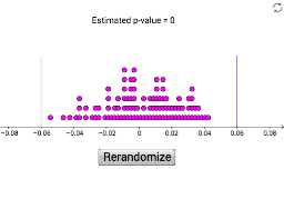
This example demonstrates how to simulate data and create a histogram to visualize the characteristics of a normal distribution. Key math concepts include Dilation, Normal Distribution, Cylinder, Arithmetic Mean, and Histogram. It utilizes GeoGebra commands and objects such as Join, Shuffle, Take, Sum, DotPlot, Segment, and variables like a, seven, eight, list1, list2, shufsev, shufeight, sumeight, sumseven, b, button1, data, list3, text1, f, g. Suitable for high school students learning probability, statistics, and data analysis.
GeoGebra Commands & Parameters
Join({Sequence[1, a, 1, 676], Sequence[0, a, 1, 1009 - 676]}) → sevenJoin({Sequence[1, a, 1, 622], Sequence[0, a, 1, 1020 - 622]}) → eightJoin({seven, eight}) → list1Shuffle(list1) → list2Take(list2, 1, 1009) → shufsevTake(list2, 1010, 2029) → shufeightSum(shufeight) → sumeightSum(shufsev) → sumsevenDotPlot(data, false, 0.4) → list3Segment((-0.06, 3), (-0.06, 0)) → fSegment((0.06, 3), (0.06, 0)) → g