
Simple Distributivity: A Geometric Visualization
Loading the math board and drawing, please wait…
In collections
Algebraic puzzles for binomial formula
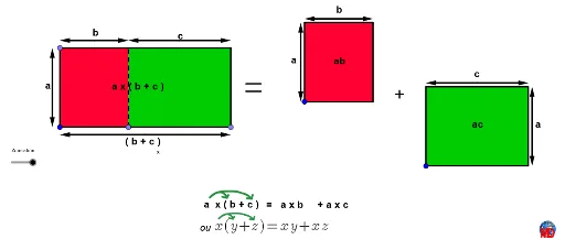
① This GeoGebra example demonstrates the distributive law (e.g., a(b+c)=ab+ac) through geometric visualization, using translations, midpoints, and polygons to compare areas or segment lengths. ② Core mathematical concepts include the distributive property, algebra-geometry correspondence, vector translation, polygon area, and geometric transformations. ③ Construction highlights: from the summary, commands such as Line, Point, Ray, Intersect, Polygon, Midpoint, Segment, Vector, and Translate are used, creating multiple points (A through R), segments, polygons (poly3, poly4), and auxiliary objects (pic1, pic2). The construction splits shapes via translations and midpoints to illustrate the distributive law. ④ Suitable for middle school to high school students, this example aids in cross-disciplinary understanding of algebra and geometry, and serves as a classroom demonstration or self-exploration tool to connect abstract algebraic rules with intuitive geometric representations.
GeoGebra Commands & Parameters
Line(A, yAxis) → g_1Line(A, xAxis) → h_1Point(g_1) → FPoint(h_1) → C_1Ray(A, F) → i_1Ray(A, C_1) → j_1Point(j_1) → BPoint(j_1) → CLine(B, i_1) → k_1Line(C, i_1) → l_1Line(F, j_1) → m_1Intersect(l_1, m_1) → DIntersect(m_1, k_1) → EPolygon(F, E, B, A) → poly3, b_2, g_2, d_2, a_2Polygon(E, D, C, B) → poly4, g_3, f_2, e_2, d_3Midpoint(E, A) → H_1Midpoint(D, B) → I_1Midpoint(I, J) → LMidpoint(H, G) → MMidpoint(J, K) → NMidpoint(f_2) → OSegment(Q, S) → aSegment(R, T) → bVector(A, U) → uVector(B, V) → vTranslate(F, Vector[(Animation * u)]) → F'Translate(E, Vector[(Animation * u)]) → E'Translate(B, Vector[(Animation * u)]) → C'Translate(A, Vector[(Animation * u)]) → A'Polygon(F', E', C', A') → poly3', f', e', c', a'Translate(E, Vector[(Animation * v)]) → E'_1Translate(D, Vector[(Animation * v)]) → D'Translate(C, Vector[(Animation * v)]) → B'Translate(B, Vector[(Animation * v)]) → C'_1Polygon(E'_1, D', B', C'_1) → poly4', e'_1, d', b', c'_1Midpoint(e') → WMidpoint(c'_1) → ZMidpoint(W, Z) → A_1Midpoint(E', A') → G_1Midpoint(D', C'_1) → J_1Midpoint(K_1, L_1) → S_1Midpoint(M_1, N_1) → T_1Midpoint(Q_1, R_1) → U_1Midpoint(O_1, P_1) → V_1Vector(N, K) → wVector(N, J) → zVector(L, J) → dVector(L, I) → eVector(M, H) → fVector(M, G) → gVector(S_1, L_1) → hVector(S_1, K_1) → iVector(V_1, O_1) → jVector(V_1, P_1) → kVector(T_1, N_1) → lVector(T_1, M_1) → mVector(U_1, Q_1) → nVector(U_1, R_1) → pMidpoint(W_1, Z_1) → A_2Vector(A_2, Z_1) → qVector(A_2, W_1) → rMidpoint(H_1, I_1) → B_2Segment(F_1, E_1) → sSegment(B_1, D_1) → t
AI Drawing Prompt Reference
Draw a geometric figure illustrating the distributive law. Start at an origin point, create two rays along perpendicular axes. On one ray, place two points; on the other, place one point. Through these points, draw parallel lines to form two adjacent rectangles. Connect key vertices with segments and mark midpoints of sides. Then translate both rectangles along two different vector directions, producing two sets of shifted rectangles. Mark midpoints of the shifted sides as well. Finally, connect these midpoints with segments to compare areas or lengths before and after translation, visually demonstrating the distributive property.
The prompt above was compiled from the original drawing commands and is for reference only.