Scalable Vectors with Optional Components

Loading the math board and drawing, please wait…

2017-02-26 20:38

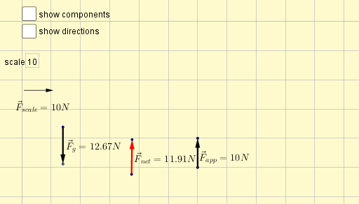
This example demonstrates the dynamic behavior and geometric representation of scalable vectors with optionally visible components. It involves core mathematical concepts such as vectors, vector magnitude, direction, component decomposition, and linear combinations. The construction utilizes GeoGebra commands and objects like Vector, OrthogonalLine, Midpoint, Textfield, Distance, Point, Line, Intersect, Angle, and Segment to build geometric elements. Suitable for high school and above students learning vector algebra, spatial geometry, and linear algebra basics, or for physics demonstrations in mechanics.

GeoGebra Commands & Parameters

Vector(A, B) → u
OrthogonalLine(A, yAxis) → f
Midpoint(A, B) → D
Textfield(scale) → InputBox1
Distance(A, B) → distanceAB
Point(u) → E
Line(A, xAxis) → g
OrthogonalLine(E, g) → h
Intersect(g, h) → C
Angle(C, A, E) → α
Segment(A, C) → i
Vector(F, G) → v
Midpoint(F, G) → H
Vector(I, J) → w
Midpoint(I, J) → K
Distance(I, J) → distanceIJ
Line(I, xAxis) → j
OrthogonalLine(K, j) → k
Intersect(j, k) → L
Segment(I, L) → l
Angle(L, I, K) → β
OrthogonalLine(M, xAxis) → m
Point(m) → N
Vector(M, N) → b
Midpoint(M, N) → O
Distance(M, N) → distanceMN
Line(R, xAxis) → n
Line(S, xAxis) → p
Line(P, yAxis) → q
Line(Q, yAxis) → r
Point(q) → T
Vector(P, T) → c
Point(r) → U
Vector(Q, U) → d
Point(n) → V
Vector(R, V) → e
Point(p) → W
Vector(S, W) → t
Midpoint(P, T) → Z
Midpoint(Q, U) → A_1
Midpoint(R, V) → B_1
Midpoint(S, W) → C_1
Distance(P, T) → distancePT
Distance(Q, U) → distanceQU
Distance(R, V) → distanceRV
Distance(S, W) → distanceSW