
Rotation vs. Time - Cube Root
Loading the math board and drawing, please wait…
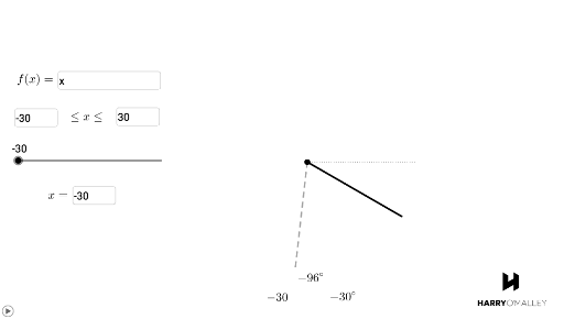
This example demonstrates the relationship between rotation and time, involving cube root functions. Using GeoGebra commands such as Rotate and Circle, it dynamically shows how rotating objects change over time. Suitable for high school mathematics education, particularly in coordinate geometry and function graphing.
GeoGebra Commands & Parameters
Textfield(f) → InputBox1Textfield(a) → InputBox2Textfield(b) → InputBox3Segment(A, B) → gRotate(A, (f(t))°, A) → A'Rotate(B, (f(t))°, A) → B'Segment(A', B') → g'Rotate(A, (h(t) / ((2 * π)) * 360), A) → A'_{1}Rotate(B, ((h(t) / 360 * 2) * π), A) → B'_{1}Segment(A'_{1}, B'_{1}) → g'_{1}Textfield(t) → InputBox4Circle(A, B) → e
AI Drawing Prompt Reference
Create a dynamic rotation diagram: a segment rotates around a fixed center point, with its angle determined by a cube root function of time. Simultaneously, another segment rotates using a different formula involving pi, creating a comparison. Both rotating segments share the same center, and a reference circle is drawn with that center passing through the segment endpoints. Include four input fields to adjust function parameters and the current time, updating the graph in real time.
The prompt above was compiled from the original drawing commands and is for reference only.