
Resistance to Outliers Demo
Loading the math board and drawing, please wait…
In collections
AP Statistics
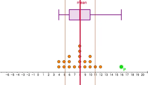
This example demonstrates how box plots and comparisons of mean vs median visually illustrate a dataset's resistance to outliers. Key math concepts include mean, median, quartiles, box plots, outliers, and data dispersion. GeoGebra commands used are Point, Sequence, DotPlot, Mean, SampleSD, Median, Q1, Q3, BoxPlot. Suitable for high school statistics and probability courses to understand data distribution and outlier effects.
GeoGebra Commands & Parameters
Point(Segment[(-5, 1), (20, 1)]) → PSequence(RandomBinomial[20, 0.35], a, 1, 20) → list1DotPlot(Append[list1, x(P)]) → list2Mean(Append[list1, x(P)]) → aSampleSD(Append[list1, x(P)]) → bMedian(Append[list1, x(P)]) → dQ1(Append[list1, x(P)]) → eQ3(Append[list1, x(P)]) → fBoxPlot(11, 1, Append[list1, x(P)]) → c