
Related Rates: Particle Traveling Problem
Loading the math board and drawing, please wait…
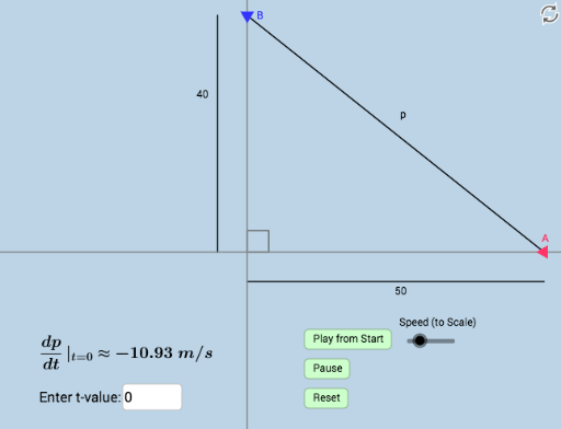
This example demonstrates a particle traveling problem, involving concepts of derivatives and related rates. Using GeoGebra commands such as Circle, Intersect, Polygon, etc., the motion of the particle and its velocity changes can be dynamically displayed. Suitable for high school mathematics teaching, particularly in calculus and derivatives.
GeoGebra Commands & Parameters
Circle(G, b) → qIntersect(q, g, 1) → B_2Intersect(q, f, 2) → A_2Polygon(A_1, A_2, B_2) → poly1, c_1, a_1, b_1Segment(B_2, A_2) → wRay(A_1, A_2) → iRay(A_1, B_2) → jDistance(A_1, B_2) → distanceACSegment(A_1, A_2) → kSegment(A_1, B_2) → lIntersect(f, xAxis) → CIntersect(f, xAxis) → EIntersect(f, xAxis) → HIntersect(q, g) → K, LSegment(A_1, L) → mIntersect(q, g, 1) → NCircle(L, 10) → d_1Intersect(d_1, g, 2) → OSegment(R, S) → h_1Segment(T, U) → i_1Ray(Z, B_1) → p_1Ray(G, C_1) → sCircle(A, 5) → cIntersect(f, xAxis) → D_1Intersect(c, y = 0) → E_1, F_1Ray(A, E_1) → tSegment(Z, A) → dCircle(W, 5) → e_1Intersect(e_1, g) → G_1, H_1Point(s) → I_1Intersect(e_1, x = 0) → I, JCircle(J, 5) → eRay(B, J) → rSegment(P, B) → aAngle(Z, A_1, P) → βSegment(B, A) → pTextfield(u) → InputBox1