Radioactive Decay Model: Exponential Attenuation with Calculus Visualization

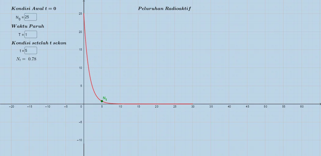
This GeoGebra example demonstrates how the amount of a radioactive substance changes over time, visualizing the exponential decay law and relating it to calculus ideas about the decay rate. Key math concepts include exponential functions (and the typical use of logarithmic relationships for understanding parameters), interactive function graphing, and the derivative as an instantaneous rate of change. Construction focuses on GeoGebra Textfield and InputBox objects to input and adjust parameters and variables such as N0, Nt, time t, and quantities like A, while the object f represents the decay function used for plotting and updating results. Additional text objects (text1–text5) label variables and display expressions/outputs to make the model interpretable. Suitable for high school and early undergraduate instruction on mathematical modeling, exponential/logarithmic functions, and calculus applications to rate-of-change visualization.