Series RLC Circuit: Impedance Components via Phasor Vectors

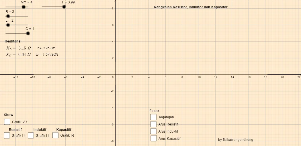
This example demonstrates how a series RLC circuit’s impedance components and current phasor relationships change with angular frequency. It visually explains the contribution of resistance, inductance, and capacitance to the overall response. Key math concepts include vector (phasor) modeling, complex-component interpretation via imaginary parts (e.g., ImL, ImC, ImR), and reactance terms such as XL and XC, all parameterized by frequency-related variables (ω, T, f, W). In GeoGebra, the construction is centered on the Vector command to build phasor vectors and assemble them into combined quantities (e.g., objects A, B and intermediate vectors u, v, w, plus labeled parameter objects like Vm, R, L, C, XL, XC, and the text annotations text1–text9). The resulting geometric relationships provide a dynamic, graphical way to study frequency-domain behavior. Suitable for classroom use and self-study in upper secondary through early university, especially for teaching phasor methods and frequency response intuition.