
Radioactive Decay Demonstration
Loading the math board and drawing, please wait…
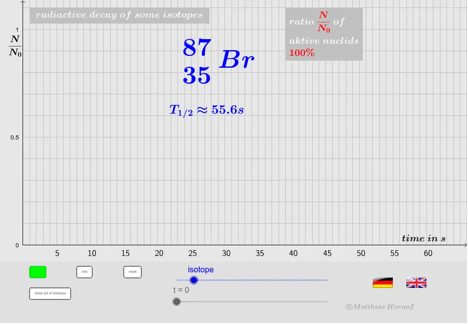
This example demonstrates the decay process of several isotopes, involving exponential functions and Poisson distribution. It uses GeoGebra commands like Function, OrthogonalLine, Intersect, and Segment, along with objects such as sliders and loci for construction. Ideal for high school students or probability & statistics and calculus education.
GeoGebra Commands & Parameters
Function(f1, 0, t / a) → f1zOrthogonalLine(Hp, yAxis) → g_1Intersect(f1, g_1, (55.59998175614492, 0.5000000000001242)) → Hp_1OrthogonalLine(Hp_2, yAxis) → g_2Intersect(f1, g_2, (111.1999635123297, 0.25)) → Hp_3OrthogonalLine(Hp_4, yAxis) → g_3Intersect(f1, g_3, (166.79994526849458, 0.12499999999999997)) → Hp_5OrthogonalLine(Hp_6, yAxis) → g_4Intersect(f1, g_4, (693.1471805599454, 0.06249999999999998)) → Hp_7Segment(Hp, Pr1h) → f1horSegment(Pr1h, Hp1u) → f1verSegment(Hp_2, Pr2h) → f2horSegment(Pr2h, Hp3u) → f2verSegment(Pr4h, Hp7u) → f4verSegment(Hp5u, Pr3h) → f3verSegment(Hp_4, Pr3h) → f3horSegment(Hp_6, Pr4h) → f4hor