Radford University GeoGebra Webinar: Calculus Visualization

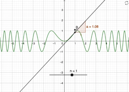
This example demonstrates how to use GeoGebra to dynamically visualize core calculus concepts, including function graphs, tangent line slopes, and the geometric meaning of definite and indefinite integrals. It uses interactive sliders and dynamic objects to show the derivative as the slope of a tangent line, the integral as accumulation of area, and the approximation of definite integrals via Riemann sums (upper and lower sums). The construction employs the Tangent command to draw the tangent line to function f at point A, the Slope command to compute its slope, and defines objects such as n (number of subdivisions), g (auxiliary function), a (lower limit), and B (upper limit) to build a dynamic integral demonstration. This example is suitable for university calculus courses or advanced high school mathematics, helping students grasp the geometric intuition of derivatives and integrals, as well as numerical approximation methods.