
Rabbit Population Growth Scatter Plot Analysis
Loading the math board and drawing, please wait…
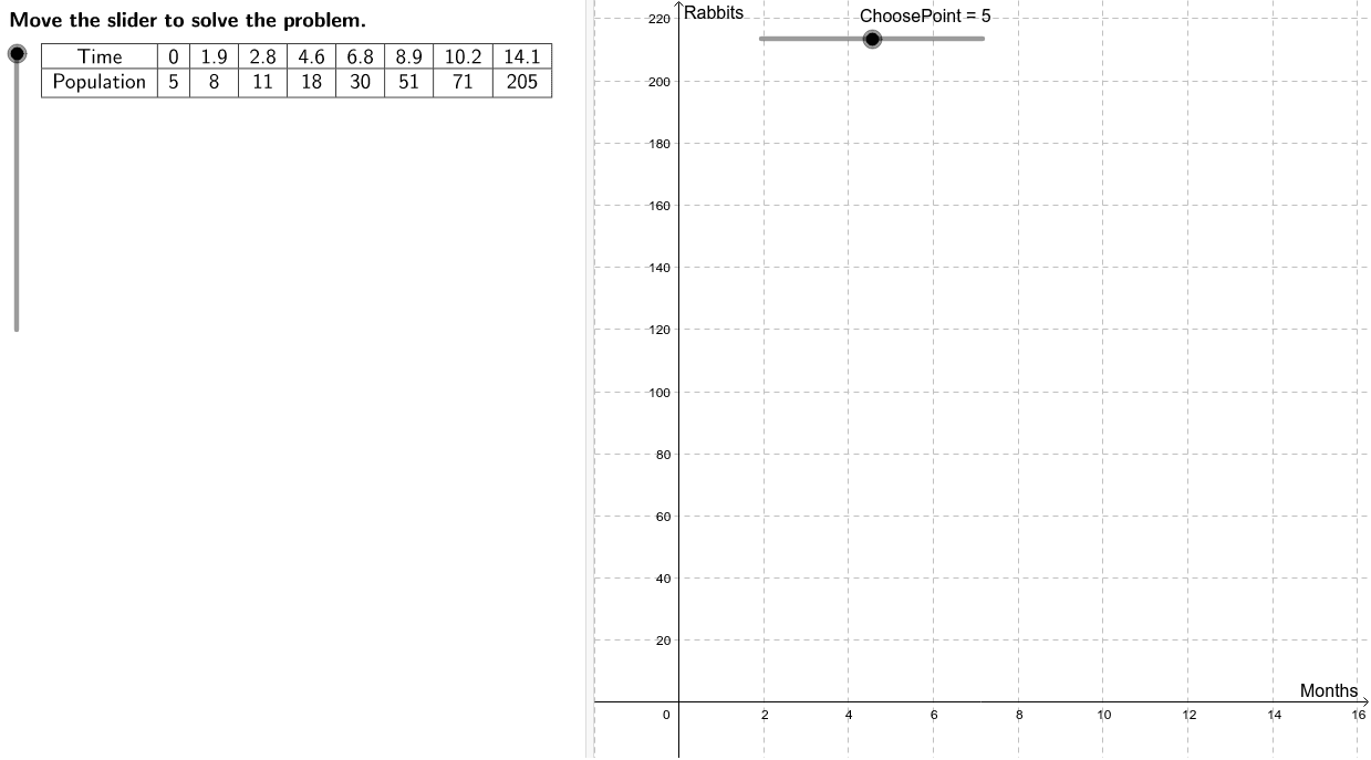
This example demonstrates the trend of rabbit population growth over time using a scatter plot. Key math concepts include data analysis, function fitting, and calculus concepts like derivatives and integrals. GeoGebra commands and objects used in the construction summary are LaTeX, table, slider, and data zooming. Suitable for high school mathematics teaching on data visualization and function modeling.
GeoGebra Commands & Parameters
LaTeX(steps) → counterLaTeX("\text{Move the slider to solve the problem.}") → text0LaTeX("\text{Use the buttons below to return to the original}\cr\text{problem or randomly generate a similar practice}\cr\text{problem.}") → RandomizationTextCorner(1) → ACorner(3) → BCell(2, ChoosePoint) → n_{model}Cell(1, ChoosePoint) → t_{model}LaTeX("\text{Create a scatter plot of the data.}") → text1LaTeX("\text{Let }\textcolor{#000099}{x}\text{ represent the number of months and }\textcolor{#000099}{y}\cr\text{represent the rabbit population.}") → text2LaTeX("\text{Write an equation that describes the function.}") → text3LaTeX("\text{The data appears to follow an exponential curve in}\cr\text{the form }\textcolor{#006633}{y = a b^x}\text{, for which }\textcolor{#006633}{a}\text{ is the y-intercept of}\cr\text{the graph.}") → text4LaTeX((((("\text{From the data table, it can be seen that the}\cr\text{y-intercept is }\textcolor{#006633}{(0, " * n_{start}) * ")}\text{. Therefore, }\textcolor{#006633}{a = ") * n_{start}) * "}.")) → text5LaTeX((((((("\text{Choose a second point from the data table such}\cr\text{as }\textcolor{#006633}{(" * t_{model}) * ", ") * n_{model}) * " )}\text{. Substitute these }\textcolor{#006633}{x}\text{ and }\textcolor{#006633}{y}\text{ values as}\cr\text{well as the value of }\textcolor{#006633}{a=") * n_{start}) * "}\text{ into the general form }\cr\textcolor{#006633}{y = a b^x}\text{ and solve for }\textcolor{#006633}{b}.")) → text6LaTeX("\text{Use the ChoosePoint slider to see how the}\cr\text{equation modeling the data depends on which}\cr\text{data point is used to solve for }\textcolor{#006633}{b}.") → text10LaTeX("\text{Create a residual plot to check if the function model}\cr\text{is a good fit for the situation.}") → text11LaTeX("\text{Plot the residuals and determine if the function is}\cr\text{a good fit for the data.}") → text18LaTeX("\text{Use the function to predict the rabbit population}\cr\text{after 16 months.}") → text20LaTeX((("\text{After 16 months, there will be approximately }\cr" * n_{16}) * "\text{ rabbits, assuming their population continues}\cr\text{to grow at this rate.}")) → text23Max({E1, E2, E3, E4, E5, E6, E7, E8}) → maxResidMin({E1, E2, E3, E4, E5, E6, E7, E8}) → minResidMax((maxResid * 1.1), maxResid + 1) → ymaxRTableText({{LaTeX["Time"], LaTeX[A1], LaTeX[A2], LaTeX[A3], LaTeX[A4], LaTeX[A5], LaTeX[A6], LaTeX[A7], LaTeX[A8]}, {LaTeX["Population"], LaTeX[B1], LaTeX[B2], LaTeX[B3], LaTeX[B4], LaTeX[B5], LaTeX[B6], LaTeX[B7], LaTeX[B8]}}, "c_|") → ProblemTableText({{LaTeX["x"], LaTeX[(((("\textcolor{#006633}{y_0=" * n_{start}) * "(") * b) * ")^x}")]}, {LaTeX[A1], LaTeX[D1]}, {LaTeX[A2], LaTeX[D2]}, {LaTeX[A3], LaTeX[D3]}, {LaTeX[A4], LaTeX[D4]}, {LaTeX[A5], LaTeX[D5]}, {LaTeX[A6], LaTeX[D6]}, {LaTeX[A7], LaTeX[D7]}, {LaTeX[A8], LaTeX[D8]}}, "c_|") → text15LaTeX("\text{Create a table of each x-value and its}\cr\text{corresponding model y-value (}\textcolor{#006633}{y_0}\text{). Round }\textcolor{#006633}{y_0}\text{ to}\cr\text{the nearest integer since it is not possible to have}\cr\text{a fraction of a rabbit.}") → text14LaTeX("\text{Find the difference between the observed value}\cr\text{and calculated value for each value of }\textcolor{#006633}{x}\text{. This}\cr\text{difference, }\textcolor{#006633}{y – y_0}\text{, is the residual.}") → text16TableText({{LaTeX["\textcolor{#006633}{x}"], LaTeX["\text{residual (}\textcolor{#006633}{y-y_0}\text{)}"]}, {LaTeX[A1], LaTeX[((((B1 * "-") * D1) * "=") * E1)]}, {LaTeX[A2], LaTeX[((((B2 * "-") * D2) * "=") * E2)]}, {LaTeX[A3], LaTeX[((((B3 * "-") * D3) * "=") * E3)]}, {LaTeX[A4], LaTeX[((((B4 * "-") * D4) * "=") * E4)]}, {LaTeX[A5], LaTeX[((((B5 * "-") * D5) * "=") * E5)]}, {LaTeX[A6], LaTeX[((((B6 * "-") * D6) * "=") * E6)]}, {LaTeX[A7], LaTeX[((((B7 * "-") * D7) * "=") * E7)]}, {LaTeX[A8], LaTeX[((((B8 * "-") * D8) * "=") * E8)]}}, "c_|") → text17LaTeX((((("\text{Since the points appear to be spread out}\cr\text{randomly, }\textcolor{#006633}{y_0 = " * n_{start}) * "(") * b) * ")^x}\text{ is a good fit for the}\cr\text{data.}")) → text19LaTeX("\text{Substitute for }\textcolor{#006633}{a}\text{ and }\textcolor{#006633}{b}\text{ in the general form }\textcolor{#006633}{y=ab^x}\text{.}\cr\text{Since }\textcolor{#006633}{y}\text{ is used for the observed values of the}\cr\text{population, use }\textcolor{#006633}{y_0}\text{ in this equation modeling the}\cr\text{data.}") → text8LaTeX((((("\textcolor{#006633}{y_0 = " * n_{start}) * "(") * b) * ")^x}")) → text9LaTeX((((("\text{The residual is the difference between the observed}\cr\text{value and the estimated value using the function }\cr\textcolor{#006633}{y_0 = " * n_{start}) * "(") * b) * ")^x}.")) → text12LaTeX((((("\text{The observed values (}\textcolor{#006633}{y}\text{) are the populations in the}\cr\text{table. The corresponding model values (}\textcolor{#006633}{y_0}\text{) are}\cr\text{determined by evaluating }\textcolor{#006633}{y_0 = " * n_{start}) * "(") * b) * ")^x}\text{ for each}\cr\text{value of }\textcolor{#006633}{x}\text{ in the data table.}")) → text13LaTeX("\text{Substitute }\textcolor{#006633}{16}\text{ for }\textcolor{#006633}{x}\text{ and evaluate to determine the}\cr\text{corresponding value for }\textcolor{#006633}{y_0}.") → text21TableText({{LaTeX["\textcolor{#006633}{y=a b^x}"], LaTeX["\text{General form}"]}, {LaTeX[(((((("\textcolor{#006633}{" * n_{model}) * "=") * n_{start}) * " b^{") * t_{model}) * "}}")], LaTeX["\text{Use values from the data.}"]}, {LaTeX[(((("\textcolor{#006633}{" * lhs) * "= b^{") * t_{model}) * "}}")], LaTeX[(("\text{Divide both sides by }\textcolor{#006633}{" * n_{start}) * "}.")]}, {LaTeX[(((("\textcolor{#006633}{\sqrt[" * t_{model}) * "]{") * lhs) * "}= b}")], LaTeX[(("\text{Take the }\textcolor{#006633}{" * t_{model}) * "}\text{th root of both sides.}")]}, {LaTeX[(("\textcolor{#006633}{b \approx " * b) * "}")], LaTeX["\text{Use a calculator to evaluate.}"]}}) → text7TableText({{LaTeX[(((("\textcolor{#000099}{y_0=" * n_{start}) * "(") * b) * ")^x}")], LaTeX["\text{Model function}"]}, {LaTeX[(((("\textcolor{#000099}{y_0=" * n_{start}) * "(") * b) * ")^{16}}")], LaTeX["\text{Substitute }\textcolor{#006633}{16}\text{ for }\textcolor{#006633}{x}."]}, {LaTeX[(("\textcolor{#000099}{y_0\approx " * n_{16}) * "}")], LaTeX["\text{Use a calculator to simplify.}"]}}) → text22
AI Drawing Prompt Reference
Create a scatter plot analyzing rabbit population growth over time, fitting an exponential curve to the data points, highlighting key points like the starting point and a chosen data point, calculating and displaying a residual plot, and predicting the population after 16 months, with all calculations and results clearly labeled on the graph.
The prompt above was compiled from the original drawing commands and is for reference only.