Pursuit Paths via Complex Numbers

Loading the math board and drawing, please wait…

2018-10-18 02:06

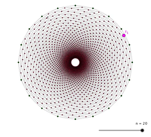
This GeoGebra example demonstrates how complex numbers can model classic pursuit path problems in dynamic geometry. Multiple agents start from vertices of a regular polygon and each agent continuously moves toward the next agent at constant speed, forming elegant closed pursuit curves. Key mathematical concepts include geometric interpretation of complex numbers, parametric equations, limits and convergence, and similarity transformations. The construction uses GeoGebra commands: Sequence to generate evenly distributed polygon vertices, Polygon to draw pursuit paths, Circle to define movement boundaries, and a slider parameter n to control the number of agents. This dynamic demonstration helps students intuitively understand how complex numbers describe planar motion and experience the mathematical transition from discrete to continuous. Suitable for high school mathematics extension courses, introductory complex analysis, and math modeling enthusiasts.

GeoGebra Commands & Parameters

Sequence((cos(w), sin(w)), w, (2 * π / n), (2 * π), (2 * π / n)) → L_1
Polygon(L_1) → t1
Polygon(A1) → B1
Polygon(A2) → B2
Polygon(A3) → B3
Polygon(A4) → B4
Polygon(A5) → B5
Polygon(A6) → B6
Polygon(A7) → B7
Polygon(A8) → B8
Polygon(A9) → B9
Polygon(A10) → B10
Polygon(A11) → B11
Polygon(A12) → B12
Polygon(A13) → B13
Polygon(A14) → B14
Polygon(A15) → B15
Polygon(A16) → B16
Polygon(A17) → B17
Polygon(A18) → B18
Polygon(A19) → B19
Polygon(A20) → B20
Polygon(A21) → B21
Polygon(A22) → B22
Polygon(A23) → B23
Polygon(A24) → B24
Polygon(A25) → B25
Polygon(A26) → B26
Polygon(A27) → B27
Polygon(A28) → B28
Polygon(A29) → B29
Polygon(A30) → B30
Polygon(A31) → B31
Polygon(A32) → B32
Polygon(A33) → B33
Polygon(A34) → B34
Polygon(A35) → B35
Polygon(A36) → B36
Polygon(A37) → B37
Polygon(A38) → B38
Polygon(A39) → B39
Polygon(A40) → B40
Polygon(A41) → B41
Polygon(A42) → B42
Polygon(A43) → B43
Polygon(A44) → B44
Polygon(A45) → B45
Polygon(A46) → B46
Polygon(A47) → B47
Polygon(A48) → B48
Polygon(A49) → B49
Polygon(A50) → B50
Polygon(A51) → B51
Polygon(A52) → B52
Polygon(A53) → B53
Polygon(A54) → B54
Polygon(A55) → B55
Polygon(A56) → B56
Polygon(A57) → B57
Polygon(A58) → B58
Polygon(A59) → B59
Polygon(A60) → B60
Polygon(A61) → B61
Polygon(A62) → B62
Polygon(A63) → B63
Polygon(A64) → B64
Polygon(A65) → B65
Polygon(A66) → B66
Polygon(A67) → B67
Polygon(A68) → B68
Polygon(A69) → B69
Polygon(A70) → B70
Polygon(A71) → B71
Polygon(A72) → B72
Polygon(A73) → B73
Polygon(A74) → B74
Polygon(A75) → B75
Polygon(A76) → B76
Polygon(A77) → B77
Polygon(A78) → B78
Polygon(A79) → B79
Polygon(A80) → B80
Polygon(A81) → B81
Polygon(A82) → B82
Polygon(A83) → B83
Polygon(A84) → B84
Polygon(A85) → B85
Polygon(A86) → B86
Polygon(A87) → B87
Polygon(A88) → B88
Polygon(A89) → B89
Polygon(A90) → B90
Polygon(A91) → B91
Polygon(A92) → B92
Polygon(A93) → B93
Polygon(A94) → B94
Polygon(A95) → B95
Polygon(A96) → B96
Polygon(A97) → B97
Polygon(A98) → B98
Polygon(A99) → B99
Polygon(A100) → B100
Circle((0, 0), 1) → c

AI Drawing Prompt Reference

Draw pursuit curves. Create an adjustable slider parameter n to control the number of agents. Generate n evenly distributed vertices on a unit circle. Starting from each vertex, each agent moves continuously at constant speed towards the next agent, forming elegant closed pursuit curves. The trajectories of multiple agents interweave to present spiral geometric patterns, demonstrating the mathematical transition from discrete to continuous.

The prompt above was compiled from the original drawing commands and is for reference only.