
Pursuit Curves: Dynamic Multi-Target Tracking Geometry
Loading the math board and drawing, please wait…
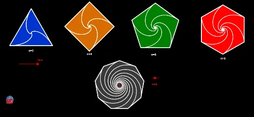
①This example demonstrates the classic 'pursuit curves' phenomenon: multiple pursuers (e.g., points B, C) chase their targets along vectors or straight lines, generating curved trajectories. ②Core mathematical concepts include vectors, parametric equations, loci, sequences, and polygon construction, touching on differential geometry of pursuit curves and iterative approximation. ③Construction highlights: from the summary, GeoGebra commands such as Vector, If, Segment, Sequence, Polygon, and Join are used, with objects including points (A, B, C, D, E, F), vectors (u, n), parameters (tmax, dd, ee, ff), and tracking objects (Trace, mice, L1-L7). Sliders or parameters control time steps to animate the pursuit paths. ④Suitable for high school to undergraduate mathematics teaching, for visualizing vector motion, parametric curves, and iterative approximation, and useful in mathematical modeling or competition extensions.
GeoGebra Commands & Parameters
Vector((1, 0)) → uIf(n ≟ 3, 26, If[n ≟ 4, 46, If[n ≟ 5, 60, 73]]) → tmaxSegment(A, B) → cSequence(s, s, 0, 6.28, 0.06283185307179587) → L1Sequence((x(O) + ((Zoom * cos(Element[L1, i] + 3.142 / 2)) * ℯ^((b * Element[L1, i]))), y(O) + ((Zoom * sin(Element[L1, i] + 3.142 / 2)) * ℯ^((b * Element[L1, i])))), i, 1, mice) → L2Sequence(Rotate[Element[L2, i], (2 * 3.14 / n), O], i, 1, Length[L2]) → L3Sequence(Sequence[Rotate[Element[L2, i], ((k * 2) * 3.14 / n), O], i, 1, Length[L2]], k, 1, n) → L4Sequence(Rotate[Element[L2, 1], ((k * 2) * 3.14 / n), O], k, 1, n + 1) → L5Sequence(Segment[Element[L5, i], Element[L5, i + 1]], i, 1, n) → L6Sequence(Rotate[Element[L2, Length[L2]], ((k * 2) * 3.14 / n), O], k, 1, n) → L7Sequence((x(C) + ((Zoom * cos(Element[L1, i] + 3.142 / 2)) * ℯ^((cc * Element[L1, i]))), y(C) + ((Zoom * sin(Element[L1, i] + 3.142 / 2)) * ℯ^((cc * Element[L1, i])))), i, 1, mice) → L2CSequence(Rotate[Element[L2C, 1], ((k * 2) * 3.14 / 3), C], k, 1, 4) → L5CSequence(Segment[Element[L5C, i], Element[L5C, i + 1]], i, 1, 3) → L6CSequence(Sequence[Rotate[Element[L2C, i], ((k * 2) * 3.14 / 3), C], i, 1, Length[L2C]], k, 1, 3) → L4CSequence((x(D) + ((Zoom * cos(Element[L1, i] + 3.142 / 2)) * ℯ^((dd * Element[L1, i]))), y(D) + ((Zoom * sin(Element[L1, i] + 3.142 / 2)) * ℯ^((dd * Element[L1, i])))), i, 1, mice) → L2DSequence(Rotate[Element[L2D, i], 1.5708, D], i, 1, Length[L2D]) → L3DSequence(Sequence[Rotate[Element[L3D, i], ((k * 2) * 3.14 / 4), D], i, 1, Length[L3D]], k, 1, 4) → L4DSequence(Rotate[Element[L3D, 1], ((k * 2) * 3.14 / 4), D], k, 1, 5) → L5DSequence(Segment[Element[L5D, i], Element[L5D, i + 1]], i, 1, 4) → L6DSequence((x(E) + ((Zoom * cos(Element[L1, i] + 3.142 / 2)) * ℯ^((ee * Element[L1, i]))), y(E) + ((Zoom * sin(Element[L1, i] + 3.142 / 2)) * ℯ^((ee * Element[L1, i])))), i, 1, mice) → L2ESequence(Rotate[Element[L2E, i], 1.2566370614359172, E], i, 1, Length[L2E]) → L3ESequence(Sequence[Rotate[Element[L3E, i], ((k * 2) * 3.14 / 5), E], i, 1, Length[L3E]], k, 1, 5) → L4ESequence(Rotate[Element[L3E, 1], ((k * 2) * 3.14 / 5), E], k, 1, 6) → L5ESequence(Segment[Element[L5E, i], Element[L5E, i + 1]], i, 1, 5) → L6ESequence((x(F) + ((Zoom * cos(Element[L1, i] + 3.142 / 2)) * ℯ^((ff * Element[L1, i]))), y(F) + ((Zoom * sin(Element[L1, i] + 3.142 / 2)) * ℯ^((ff * Element[L1, i])))), i, 1, mice) → L2FSequence(Rotate[Element[L2F, i], 1.0471975511965976, F], i, 1, Length[L2F]) → L3FSequence(Sequence[Rotate[Element[L3F, i], ((k * 2) * 3.14 / 6), F], i, 1, Length[L3F]], k, 1, 6) → L4FSequence(Rotate[Element[L3F, 1], ((k * 2) * 3.14 / 6), F], k, 1, 7) → L5FSequence(Segment[Element[L5F, i], Element[L5F, i + 1]], i, 1, 6) → L6FSequence(Segment[Element[L2C, i], Element[L2C, i + 1]], i, 1, Length[L2C]) → L2CCPolygon(L5) → poly1Polygon(L5C) → poly2Polygon(L5E) → poly3Polygon(L5D) → poly4Polygon(L5F) → poly5Join(L4C) → list1Sequence(Segment[Element[L2C, i], Element[L2C, i + 1]], i, 1, Length[L2C]) → Seg2Sequence(Sequence[Rotate[Element[Seg2, i], ((k * 2) * 3.14 / 3), C], i, 1, Length[Seg2]], k, 1, 3) → L4CuSequence(Segment[Element[L2D, i], Element[L2D, i + 1]], i, 1, Length[L2D]) → Seg3Sequence(Sequence[Rotate[Element[Seg3, i], ((k * 2) * 3.14 / 4), D], i, 1, Length[Seg3]], k, 1, 4) → L4DuSequence(Segment[Element[L2E, i], Element[L2E, i + 1]], i, 1, Length[L2E]) → Seg4Sequence(Sequence[Rotate[Element[Seg4, i], ((k * 2) * 3.14 / 5), E], i, 1, Length[Seg4]], k, 1, 5) → L4EuSequence(Segment[Element[L2F, i], Element[L2F, i + 1]], i, 1, Length[L2F]) → Seg5Sequence(Sequence[Rotate[Element[Seg5, i], ((k * 2) * 3.14 / 6), F], i, 1, Length[Seg5]], k, 1, 6) → L4FuSequence(Segment[Element[L2, i], Element[L2, i + 1]], i, 1, Length[L2]) → Seg6Sequence(Sequence[Rotate[Element[Seg6, i], ((k * 2) * 3.14 / n), O], i, 1, Length[Seg6]], k, 1, n) → L4u
AI Drawing Prompt Reference
Draw a dynamic multi-target pursuit geometry: multiple pursuers move along logarithmic spiral curves from a central origin, with each curve controlled by rotation angles and scaling factors. The figure includes several regular polygons (triangle, quadrilateral, pentagon, hexagon) whose vertices are connected by endpoints of rotated spiral curves. All curves rotate symmetrically around the center or their own vertices, forming nested spiral trajectories. The overall structure is radial and symmetric, with curves extending outward from the center and clear polygon boundaries, illustrating vector motion and iterative approximation of parametric curves.
The prompt above was compiled from the original drawing commands and is for reference only.