
Properties of a Parallelogram by Philip Collett
Loading the math board and drawing, please wait…
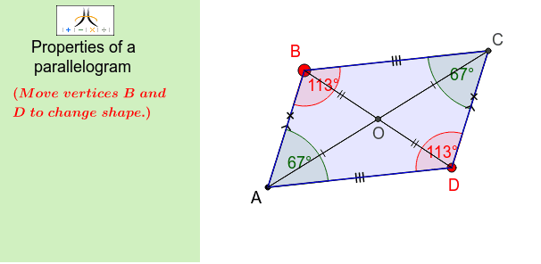
This example demonstrates the properties of a parallelogram, involving concepts such as vectors, angles, and line segments. Using GeoGebra commands like Polygon, PointIn, Line, etc., dynamic exploration of the sides, angles, and diagonals of a parallelogram is possible. Suitable for middle school and above students and teachers.
GeoGebra Commands & Parameters
Polygon(J, K, L, M) → poly2, j_1, k_1, l_1, m_1PointIn(poly2) → NLine(A, D) → lPointIn(poly2) → BAngularBisector(B, A, D) → dSegment(D_1, E_1) → eIntersect(e, d) → F_1AngularBisector(D, A, B) → kCorner(1, 1) → Cnr1Corner(1, 2) → Cnr2Corner(1, 3) → Cnr3Corner(1, 4) → Cnr4Polygon(CN1, CN2, CN3, CN4) → Panel, cn1, cn2, cn3, cn4Angle(B, D, A) → γAngle(A, B, D) → εLine(B, l) → aOrthogonalLine(A, l) → bIntersect(a, b) → EOrthogonalLine(D, l) → cIntersect(a, c) → FSegment(A, B) → fLine(D, f) → gIntersect(a, g) → CSegment(E, F) → hSegment(B, C) → iSegment(D, F) → mSegment(A, E) → nSegment(A, D) → pAngle(F, D, A) → αAngle(A, E, F) → βSegment(D, C) → jPolygon(A, E, F, D) → poly1, a_1, g_1, h_1, c_1Polygon(A, B, C, D) → poly3, a_2, b_1, i_1, c_2Segment(A, C) → qSegment(B, D) → rIntersect(q, r) → OSegment(A, O) → sSegment(O, C) → tSegment(B, O) → d_1Segment(O, D) → e_1Angle(D, A, B) → δAngle(B, C, D) → ζAngle(A, B, C) → ηAngle(C, D, A) → θPoint(f) → GPoint(j) → H