Power Law Relationship

Loading the math board and drawing, please wait…

2020-02-17 00:13

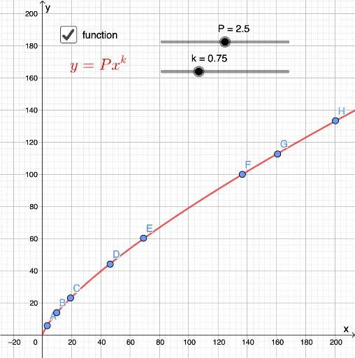
This example demonstrates the relationship between logarithmic transformation and power law. By adjusting parameters, you can observe the changes in the graphs of different power law functions. Key mathematical concepts include power law functions and logarithmic transformations. It uses points, lines, and functions in GeoGebra for construction. Suitable for high school and above students to learn the properties and graph characteristics of power law functions.

GeoGebra Commands & Parameters

Point A(3.2239524357928167, 5.8272135493670145)
Point B(9.680575476382, 13.904603272293116)
Point C(19.150289269246137, 23.035565567774793)
Point D(46.268106039720706, 44.10701701888636)
Point E(69.08150744980249, 60.26179646473856)
Point F(136.66082860796928, 99.946363364332)
Point G(160.7655546261689, 112.58923423499894)
Point H(200.36617594178256, 133.309494828592)
{A, B, C, D, E, F, G, H}
(lg(x(L_1)), lg(y(L_1)))
Numeric P(2.5)
Numeric k(0.75)
f(x) = (P * x^(k))
g(x) = (k * x) + lg(P)
Boolean a(true)
Boolean b(false)

AI Drawing Prompt Reference

Draw a graph demonstrating the relationship between logarithmic transformation and power law, including eight scattered points and two function curves: one is a power law function fitted through the points, and the other is a linear function derived from the logarithmic transformation of the power law. The scattered points are in the first quadrant, with the power law curve rising from lower left to upper right, and the linear function also showing an upward trend.

The prompt above was compiled from the original drawing commands and is for reference only.