
Logarithm as Time in Geometry
Loading the math board and drawing, please wait…
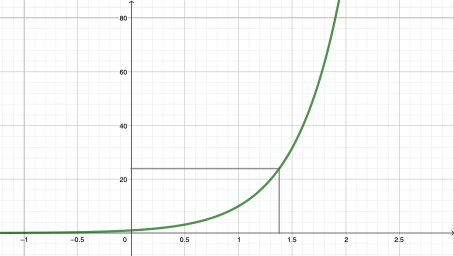
This example demonstrates the concept of logarithm through geometric representations, emphasizing the relationship between logarithm and time. Key mathematical concepts include logarithmic functions and their properties. Using GeoGebra commands such as Sequence, Point, and Segment, the example constructs the graph of a logarithmic function and related geometric elements. Suitable for high school mathematics education, it helps students understand the continuity and variation of logarithmic functions.
GeoGebra Commands & Parameters
Sequence(Segment[(k, 0), (k, 0.5)], k, -10, 10) → l1, {0.5, 0.5, 0.5, 0.5, 0.5, 0.5, 0.5, 0.5, 0.5, 0.5, 0.5, 0.5, 0.5, 0.5, 0.5, 0.5, 0.5, 0.5, 0.5, 0.5, 0.5}Sequence((log(10, k), 0), k, 1, 9) → l2, {(0, 0), (0.30102999566398114, 0), (0.47712125471966244, 0), (0.6020599913279623, 0), (0.6989700043360187, 0), (0.7781512503836435, 0), (0.8450980400142567, 0), (0.9030899869919434, 0), (0.9542425094393249, 0)}Sequence(Translate[l2, Vector[(0, 0), (k, 0)]], k, -10, 9) → m1, {{(-10, 0), (-9.698970004336019, 0), (-9.522878745280337, 0), (-9.397940008672037, 0), (-9.301029995663981, 0), (-9.221848749616356, 0), (-9.154901959985743, 0), (-9.096910013008056, 0), (-9.045757490560675, 0)}, {(-9, 0), (-8.698970004336019, 0), (-8.522878745280337, 0), (-8.397940008672037, 0), (-8.301029995663981, 0), (-8.221848749616356, 0), (-8.154901959985743, 0), (-8.096910013008056, 0), (-8.045757490560675, 0)}, {(-8, 0), (-7.698970004336019, 0), (-7.522878745280337, 0), (-7.3979400086720375, 0), (-7.301029995663981, 0), (-7.221848749616356, 0), (-7.154901959985743, 0), (-7.096910013008056, 0), (-7.045757490560675, 0)}, {(-7, 0), (-6.698970004336019, 0), (-6.522878745280337, 0), (-6.3979400086720375, 0), (-6.301029995663981, 0), (-6.221848749616356, 0), (-6.154901959985743, 0), (-6.096910013008056, 0), (-6.045757490560675, 0)}, {(-6, 0), (-5.698970004336019, 0), (-5.522878745280337, 0), (-5.3979400086720375, 0), (-5.301029995663981, 0), (-5.221848749616356, 0), (-5.154901959985743, 0), (-5.096910013008056, 0), (-5.045757490560675, 0)}, {(-5, 0), (-4.698970004336019, 0), (-4.522878745280337, 0), (-4.3979400086720375, 0), (-4.301029995663981, 0), (-4.221848749616356, 0), (-4.154901959985743, 0), (-4.096910013008056, 0), (-4.045757490560675, 0)}, {(-4, 0), (-3.6989700043360187, 0), (-3.5228787452803374, 0), (-3.3979400086720375, 0), (-3.3010299956639813, 0), (-3.2218487496163566, 0), (-3.154901959985743, 0), (-3.0969100130080567, 0), (-3.0457574905606752, 0)}, {(-3, 0), (-2.6989700043360187, 0), (-2.5228787452803374, 0), (-2.3979400086720375, 0), (-2.3010299956639813, 0), (-2.2218487496163566, 0), (-2.154901959985743, 0), (-2.0969100130080567, 0), (-2.0457574905606752, 0)}, {(-2, 0), (-1.6989700043360187, 0), (-1.5228787452803376, 0), (-1.3979400086720377, 0), (-1.3010299956639813, 0), (-1.2218487496163566, 0), (-1.1549019599857433, 0), (-1.0969100130080567, 0), (-1.0457574905606752, 0)}, {(-1, 0), (-0.6989700043360189, 0), (-0.5228787452803376, 0), (-0.3979400086720377, 0), (-0.30102999566398125, 0), (-0.22184874961635648, 0), (-0.1549019599857433, 0), (-0.09691001300805657, 0), (-0.04575749056067513, 0)}, {(0, 0), (0.30102999566398114, 0), (0.47712125471966244, 0), (0.6020599913279623, 0), (0.6989700043360187, 0), (0.7781512503836435, 0), (0.8450980400142567, 0), (0.9030899869919434, 0), (0.9542425094393249, 0)}, {(1, 0), (1.3010299956639813, 0), (1.4771212547196624, 0), (1.6020599913279623, 0), (1.6989700043360187, 0), (1.7781512503836434, 0), (1.8450980400142567, 0), (1.9030899869919433, 0), (1.9542425094393248, 0)}, {(2, 0), (2.3010299956639813, 0), (2.4771212547196626, 0), (2.6020599913279625, 0), (2.6989700043360187, 0), (2.7781512503836434, 0), (2.845098040014257, 0), (2.9030899869919433, 0), (2.9542425094393248, 0)}, {(3, 0), (3.3010299956639813, 0), (3.4771212547196626, 0), (3.6020599913279625, 0), (3.6989700043360187, 0), (3.7781512503836434, 0), (3.845098040014257, 0), (3.9030899869919433, 0), (3.9542425094393248, 0)}, {(4, 0), (4.301029995663981, 0), (4.477121254719663, 0), (4.6020599913279625, 0), (4.698970004336019, 0), (4.778151250383644, 0), (4.845098040014257, 0), (4.903089986991944, 0), (4.954242509439325, 0)}, {(5, 0), (5.301029995663981, 0), (5.477121254719663, 0), (5.6020599913279625, 0), (5.698970004336019, 0), (5.778151250383644, 0), (5.845098040014257, 0), (5.903089986991944, 0), (5.954242509439325, 0)}, {(6, 0), (6.301029995663981, 0), (6.477121254719663, 0), (6.6020599913279625, 0), (6.698970004336019, 0), (6.778151250383644, 0), (6.845098040014257, 0), (6.903089986991944, 0), (6.954242509439325, 0)}, {(7, 0), (7.301029995663981, 0), (7.477121254719663, 0), (7.6020599913279625, 0), (7.698970004336019, 0), (7.778151250383644, 0), (7.845098040014257, 0), (7.903089986991944, 0), (7.954242509439325, 0)}, {(8, 0), (8.301029995663981, 0), (8.477121254719663, 0), (8.602059991327963, 0), (8.698970004336019, 0), (8.778151250383644, 0), (8.845098040014257, 0), (8.903089986991944, 0), (8.954242509439325, 0)}, {(9, 0), (9.301029995663981, 0), (9.477121254719663, 0), (9.602059991327963, 0), (9.698970004336019, 0), (9.778151250383644, 0), (9.845098040014257, 0), (9.903089986991944, 0), (9.954242509439325, 0)}}Point(m1) → P1Segment(Q1, R1) → i1Segment(R1, S1) → j1Sequence(Segment[(log(10, k), 0), (log(10, k), 0.4)], k, 2, 9) → l3, {0.4, 0.4, 0.4, 0.4, 0.4, 0.4, 0.4, 0.4}Sequence(Translate[l3, Vector[(0, 0), (k, 0)]], k, -10, 9) → m2, {{0.4, 0.4, 0.4, 0.4, 0.4, 0.4, 0.4, 0.4}, {0.4, 0.4, 0.4, 0.4, 0.4, 0.4, 0.4, 0.4}, {0.4, 0.4, 0.4, 0.4, 0.4, 0.4, 0.4, 0.4}, {0.4, 0.4, 0.4, 0.4, 0.4, 0.4, 0.4, 0.4}, {0.4, 0.4, 0.4, 0.4, 0.4, 0.4, 0.4, 0.4}, {0.4, 0.4, 0.4, 0.4, 0.4, 0.4, 0.4, 0.4}, {0.4, 0.4, 0.4, 0.4, 0.4, 0.4, 0.4, 0.4}, {0.4, 0.4, 0.4, 0.4, 0.4, 0.4, 0.4, 0.4}, {0.4, 0.4, 0.4, 0.4, 0.4, 0.4, 0.4, 0.4}, {0.4, 0.4, 0.4, 0.4, 0.4, 0.4, 0.4, 0.4}, {0.4, 0.4, 0.4, 0.4, 0.4, 0.4, 0.4, 0.4}, {0.4, 0.4, 0.4, 0.4, 0.4, 0.4, 0.4, 0.4}, {0.4, 0.4, 0.4, 0.4, 0.4, 0.4, 0.4, 0.4}, {0.4, 0.4, 0.4, 0.4, 0.4, 0.4, 0.4, 0.4}, {0.4, 0.4, 0.4, 0.4, 0.4, 0.4, 0.4, 0.4}, {0.4, 0.4, 0.4, 0.4, 0.4, 0.4, 0.4, 0.4}, {0.4, 0.4, 0.4, 0.4, 0.4, 0.4, 0.4, 0.4}, {0.4, 0.4, 0.4, 0.4, 0.4, 0.4, 0.4, 0.4}, {0.4, 0.4, 0.4, 0.4, 0.4, 0.4, 0.4, 0.4}, {0.4, 0.4, 0.4, 0.4, 0.4, 0.4, 0.4, 0.4}}Segment((x(P1), -2), (x(P1), 2)) → h1'Point(h1') → P1'Segment((x(P1), -0.5), (x(P1), 0.8)) → h1Point(m1) → P2Segment((x(P2), -0.5), (x(P2), 0.8)) → h2Segment((x(P2), -2), (x(P2), 2)) → h2'Segment(Q2, R2) → i2Segment(R2, S2) → j2Point(h2') → P2'Point(m1) → P3Segment((x(P3), -0.5), (x(P3), 0.8)) → h3Segment((x(P3), -2), (x(P3), 2)) → h3'Point(h3') → P3'Segment(Q3, R3) → i3Segment(R3, S3) → j3Point(g) → P4Segment((x(P4), -0.5), (x(P4), 0.8)) → h4Segment(Q4, R4) → i4Segment(R4, S4) → j4
AI Drawing Prompt Reference
Draw a geometric representation of a logarithmic function to illustrate the relationship between logarithms and time. Start by drawing a series of horizontal line segments, then plot points at logarithmic intervals and translate them horizontally. Next, sketch the logarithmic function using these points, adding vertical segments and auxiliary lines to highlight its properties. Finally, include helper line segments at key points on the function to emphasize its continuity and variation.
The prompt above was compiled from the original drawing commands and is for reference only.