
Polyhedron Calculation with a Fixed Vertex on a Sphere
Loading the math board and drawing, please wait…
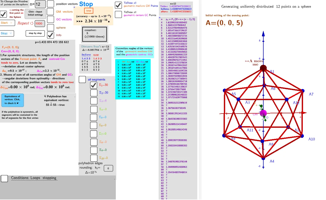
This example demonstrates how to construct a polyhedron with one vertex fixed on a sphere. It involves core mathematical concepts such as spherical geometry, polyhedron construction, vector operations, and optimization problems. Key GeoGebra commands and objects used in the construction include Sphere, Text, TableText, Sum, and Sequence. It is suitable for high school students and mathematics enthusiasts exploring solid geometry.
GeoGebra Commands & Parameters
Text("" + Um1) → txt_pLaTeX(Um1) → lll1_1LaTeX(Um0) → lll0Sphere(O, R) → p1Textfield(n) → InputBox1Textfield(i0) → InputBox2Text(r) → TxtrTextfield(k_1) → InputBox4UnicodeToLetter(34) → u34Textfield(k_2) → InputBox5TableText(ltxt0, ltxt1, "v") → textltxt01Text(("(up\; to\; 10^{-15})\;\\ accuracy= " * ScientificText[cc, 3]), C, true, true) → text5rZip(Vector[a, a + UnitVector[a]], a, lP') → lVector1Textfield(scale) → InputBox6TableText(Append["i", 1…n], Append[" \fgcolor{orange}{GM :Δφ_i}, rad", l1], Append["\fgcolor{magenta}{GC :Δφ_i} , rad", l1c], "v") → text23If(bu, "Animation", "Stop") → bue0Zip(Vector[a, a + (1.5 * UnitVector[b])], a, lP', b, Wi_P) → lVector3Zip(Vector[a, a + (1.5 * UnitVector[b])], a, lP', b, Wi_Pc) → lVector2TableText({Join[{{"n"}, Sequence[i, i, 4, 69 + 3]}], Join[{{" p_n=P_n/[R*n*(n-1)/2]"}, lp}]}, "vl") → txt_lpSum(Flatten[Sequence[Append[Sequence[Element[txt_p, i], i, m1(k), m2(k)], " "], k, 1, 5]]) → txtUm1Text("\;\;\;\;\;\;\;\;\;\;\;\;\;\fgcolor{" + (If[c', "orange", "brown"]) + "} \boxed{ " + c' + ("}\;\;\;\; \;\;\;\;\; \\\;\; ( accuracy- up\; to\;\; 2.*10^{" - k_2) + ("\;})\;\\\;\; ➤➤➤\;\;\;\scalebox{1.5}{ " + (ScientificText[cc, 3])) + "}\;█ ", C, true, true) → text9Sequence(Text["" + (i), Wi_Pc1(i) - (0.4, 0.4), true, true], i, 1, n) → l4bSequence(Text["" + (i), Wi_Pc2(i) + (0.4, 0.4), true, true], i, 1, n) → l4aAppend(As, Sequence[((random(), random(), random()) * R), i, 2, n]) → l2sPointIn(p1) → ASequence(Text["A" + (i), lP'(i) - (-0.6, 0.6), true, true], i, 1, n) → l4ccZip(Segment[Element[lP', y(a)], Element[lP', z(a)]], a, ll1bb(1)) → ll1Zip(Segment[Element[lP', y(a)], Element[lP', z(a)]], a, ll1bb(2)) → ll2Zip(Segment[Element[lP', y(a)], Element[lP', z(a)]], a, ll1bb(3)) → ll3
AI Drawing Prompt Reference
In a 3D scene, draw a sphere centered at O with radius R, and place one fixed vertex A on the sphere. Using given parameters such as n and other inputs (e.g., i0, k_1, k_2, and scale), construct a sequence of additional points on the sphere that extends from A, forming a set of numbered vertices (label them A1 through An). Display the connectivity implied by the construction by drawing the corresponding line segments between consecutive or paired vertices, producing a polyhedron-like outline on the sphere surface. Add on-canvas text and a small table showing values related to Δφ_i with GM and GC, as well as a normalized p_n value, and include a boxed accuracy/precision message indicating an accuracy bound.
The prompt above was compiled from the original drawing commands and is for reference only.