
Polar Area by Doug Kuhlmann
Loading the math board and drawing, please wait…
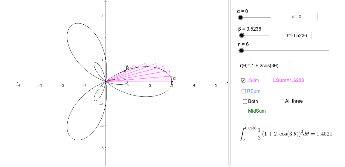
This example demonstrates how to plot polar area graphs, visualizing the regions of sine and tangent functions in polar coordinates. It involves core math concepts like polar coordinate systems, area calculation, trigonometric properties, standard deviation, and addition. GeoGebra commands and objects used include Cartesian curve plotting, sequence generation, Zip, text fields, first/last extraction, summation, and integration. Suitable for high school and above students to understand the construction of polar graphs and the visualization of function area relationships.
GeoGebra Commands & Parameters
CurveCartesian((r(θ) * cos(θ)), (r(θ) * sin(θ)), θ, 0, 6.283185307179586) → cSequence(c(α + (i * Δθ)), i, 0, n) → ThetaPtsZip(CircleSector[(0, 0), C, D], C, First[ThetaPts, n], D, Last[ThetaPts, n]) → LSecsTextfield(r) → rOFthetaTextfield(α) → αEqTextfield(β) → βEqLast(ThetaPts, n) → RptFirst(ThetaPts, n) → LptZip((Length[A]; Angle[B]), A, Rpt, B, Lpt) → RtptsZip(CircleSector[(0, 0), E, F], E, Rtpts, F, Last[ThetaPts, n]) → RSecsSum(Sequence[((0.5 * r(α + (i * Δθ))^(2)) * Δθ), i, 0, n - 1]) → LSumSum(Sequence[((0.5 * r(α + (i * Δθ))^(2)) * Δθ), i, 1, n]) → RSumSequence(c(α + ((i - 1 / 2) * Δθ)), i, 1, n) → MidθptsSum(Zip[((0.5 * R^(2)) * Δθ), R, Midθpts]) → MSumZip((Length[A]; Angle[B]), A, Midθpts, B, First[ThetaPts, n]) → MminusZip((Length[A]; Angle[B]), A, Midθpts, B, Last[ThetaPts, n]) → MplusZip(CircleSector[(0, 0), E, F], E, Mminus, F, Mplus) → MSecsIntegral(g, α, β) → Int