
Graphing Hyperbolic Cosine Function
Loading the math board and drawing, please wait…
In collections
Phantom Graphs
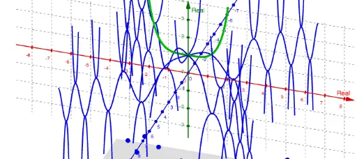
This example demonstrates how to plot the graph of the hyperbolic cosine function cosh(x^2/2) and visualize its behavior as x changes. Key mathematical concepts include hyperbolic functions, coordinate geometry, and function graphing. The construction utilizes GeoGebra commands and objects such as Plane, CurveCartesian, and Sequence. Suitable for high school and above students to understand the plotting and properties of complex function graphs.
GeoGebra Commands & Parameters
Plane((0, c, 0), (1, c, 0), (0, c, 1)) → pCurveCartesian(0, cosh(t^(2) / 2), t, t, -5, 5) → aCurveCartesian(t, cos(t^(2)), t, t, -5, 5) → bCurveCartesian(t, cos(t^(2)), (-t), t, -5, 5) → dSequence((sqrt(acos(c) + ((2 * π) * k)), c, sqrt(acos(c) + ((2 * π) * k))), k, 0, 5) → Pts_1Sequence(((-sqrt(acos(c) + ((2 * π) * k))), c, sqrt(acos(c) + ((2 * π) * k))), k, 0, 5) → Pts_3Sequence(((-sqrt(acos(c) + ((2 * π) * k))), c, (-sqrt(acos(c) + ((2 * π) * k)))), k, 0, 5) → Pts_4Sequence((sqrt(acos(c) + ((2 * π) * k)), c, (-sqrt(acos(c) + ((2 * π) * k)))), k, 0, 5) → Pts_2Sequence((sqrt((-acos(c)) + ((2 * π) * k)), c, sqrt((-acos(c)) + ((2 * π) * k))), k, 0, 5) → Pts_5Sequence((sqrt((-acos(c)) + ((2 * π) * k)), c, (-sqrt((-acos(c)) + ((2 * π) * k)))), k, 0, 5) → Pts_6Sequence(((-sqrt((-acos(c)) + ((2 * π) * k))), c, sqrt((-acos(c)) + ((2 * π) * k))), k, 0, 5) → Pts_7Sequence(((-sqrt((-acos(c)) + ((2 * π) * k))), c, (-sqrt((-acos(c)) + ((2 * π) * k)))), k, 0, 5) → Pts_8Sequence((sqrt(acosh(((-1)^(k) * c)) + sqrt(acosh(((-1)^(k) * c))^(2) + (k^(2) * π^(2)))), c, (k * π / sqrt(acosh(((-1)^(k) * c)) + sqrt(acosh(((-1)^(k) * c))^(2) + (k^(2) * π^(2)))))), k, 1, 5) → Pts_9Sequence((sqrt(acosh(((-1)^(k) * c)) + sqrt(acosh(((-1)^(k) * c))^(2) + (k^(2) * π^(2)))), c, ((-k) * π / sqrt(acosh(((-1)^(k) * c)) + sqrt(acosh(((-1)^(k) * c))^(2) + (k^(2) * π^(2)))))), k, 1, 5) → Pts_{10}Sequence(((-sqrt(acosh(((-1)^(k) * c)) + sqrt(acosh(((-1)^(k) * c))^(2) + (k^(2) * π^(2))))), c, (k * π / sqrt(acosh(((-1)^(k) * c)) + sqrt(acosh(((-1)^(k) * c))^(2) + (k^(2) * π^(2)))))), k, 1, 5) → Pts_{11}Sequence(((-sqrt(acosh(((-1)^(k) * c)) + sqrt(acosh(((-1)^(k) * c))^(2) + (k^(2) * π^(2))))), c, ((-k) * π / sqrt(acosh(((-1)^(k) * c)) + sqrt(acosh(((-1)^(k) * c))^(2) + (k^(2) * π^(2)))))), k, 1, 5) → Pts_{12}Sequence((sqrt((-acosh(((-1)^(k) * c))) + sqrt(acosh(((-1)^(k) * c))^(2) + (k^(2) * π^(2)))), c, (k * π / sqrt((-acosh(((-1)^(k) * c))) + sqrt(acosh(((-1)^(k) * c))^(2) + (k^(2) * π^(2)))))), k, 1, 5) → Pts_{13}Sequence((sqrt((-acosh(((-1)^(k) * c))) + sqrt(acosh(((-1)^(k) * c))^(2) + (k^(2) * π^(2)))), c, ((-k) * π / sqrt((-acosh(((-1)^(k) * c))) + sqrt(acosh(((-1)^(k) * c))^(2) + (k^(2) * π^(2)))))), k, 1, 5) → Pts_{14}Sequence(((-sqrt((-acosh(((-1)^(k) * c))) + sqrt(acosh(((-1)^(k) * c))^(2) + (k^(2) * π^(2))))), c, (k * π / sqrt((-acosh(((-1)^(k) * c))) + sqrt(acosh(((-1)^(k) * c))^(2) + (k^(2) * π^(2)))))), k, 1, 5) → Pts_{15}Sequence(((-sqrt((-acosh(((-1)^(k) * c))) + sqrt(acosh(((-1)^(k) * c))^(2) + (k^(2) * π^(2))))), c, ((-k) * π / sqrt((-acosh(((-1)^(k) * c))) + sqrt(acosh(((-1)^(k) * c))^(2) + (k^(2) * π^(2)))))), k, 1, 5) → Pts_{16}Sequence(CurveCartesian[t, ((-1)^(k) * cosh((0.5 * (t^(2) - (k^(2) * π^(2) / t^(2)))))), (k * π / t), t, -5, 5], k, 1, 7) → Curves1Sequence(CurveCartesian[t, ((-1)^(k) * cosh((0.5 * (t^(2) - (k^(2) * π^(2) / t^(2)))))), ((-k) * π / t), t, -5, 5], k, 1, 7) → Curves2