
Duality of Cosine and Cosh in Projective Geometry
Loading the math board and drawing, please wait…
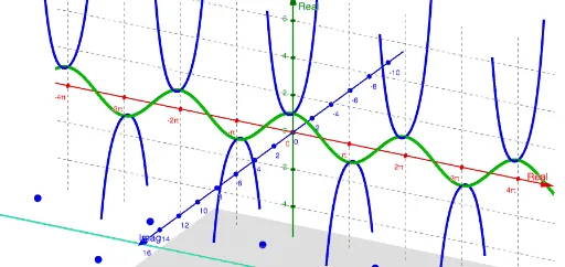
This example demonstrates the duality relationship between the cosine and hyperbolic cosine functions within projective geometry. Key mathematical concepts include trigonometric functions, hyperbolic functions, area calculations, and isosceles triangles. Construction utilizes GeoGebra commands like Sequence to generate point sets, Plane for the coordinate system, and curve objects to visualize the geometric relationships. Suitable for high school students, math enthusiasts, and educators seeking visual aids for advanced geometry and function theory.
GeoGebra Commands & Parameters
Plane((0, c, 0), (1, c, 1), (-1, c, 3)) → bSequence(((n * π), c, acosh(c)), n, -6, 6, 2) → Pts1Sequence(((n * π), c, (-acosh(c))), n, -6, 6, 2) → Pts2Sequence(((n * π), c, acosh(abs(c))), n, -5, 7, 2) → Pts3Sequence(((n * π), c, (-acosh(abs(c)))), n, -5, 7, 2) → Pts4Sequence(((n * π), acosh(c)), n, -6, 6, 2) → L_6Sequence(((n * π), (-acosh(c))), n, -6, 6, 2) → L_7Sequence(((n * π), acosh(abs(c))), n, -5, 7, 2) → L_8Sequence(((n * π), (-acosh(abs(c)))), n, -5, 7, 2) → L_9Sequence(CurveCartesian[(n * π), ((-1)^(n) * cosh(t)), t, t, -25, 25], n, -5, 5) → CurvesSequence((acos(c) + ((2 * k) * π), c), k, -10, 10) → L_1Sequence((((2 * k) * π) - acos(c), c), k, -10, 10) → L_2