
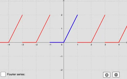
Fourier Series Demonstration
Loading the math board and drawing, please wait…
In collections
UQ-Applied Mathematical Analysis
This example demonstrates how to approximate a given function using Fourier series; core math concepts include Fourier series, trigonometric functions, and function approximation; construction highlights involve GeoGebra commands like Midpoint, Textfield, Sequence, Append, and Sum to build Fourier coefficients and function approximation graphs; suitable for high school and above mathematics learners to understand the application and principles of Fourier series and function approximation.
GeoGebra Commands & Parameters
Midpoint(A, B) → CTextfield(f) → InputBox1Textfield(initial) → InputBox2Textfield(final) → InputBox3Sequence((1 / (period / 2) * Integral[(f(x) * cos(((i * x) * π / (period / 2)))), initial, final]), i, 1, 20) → anSequence((1 / (period / 2) * Integral[(f(x) * sin(((i * x) * π / (period / 2)))), initial, final]), i, 1, 20) → bnSequence((1 / (period / 2) * Integral[(f(x) * cos(((i * x) * π / (period / 2)))), initial, final]), i, 2, 20) → an'Sequence((1 / (period / 2) * Integral[(f(x) * sin(((i * x) * π / (period / 2)))), initial, final]), i, 2, 20) → bn'Append(A1, an') → an''Append(B1, bn') → bn''Sequence((Element[an'', i] * cos(((π * i / (period / 2)) * x))) + (Element[bn'', i] * sin(((π * i / (period / 2)) * x))), i, 1, 20) → list2Textfield(A0) → InputBox4Textfield(A1) → InputBox5Textfield(B1) → InputBox6Textfield(n) → InputBox7Append(A0 / 2, list2) → list3Sequence((Element[an, i] * cos(((π * i / (period / 2)) * x))) + (Element[bn, i] * sin(((π * i / (period / 2)) * x))), i, 1, 20) → list1Sum(list3, n + 1) → p