
Pipettes: Interactive Geometry for Hypothesis Testing, Vectors, and Integral Cal
Loading the math board and drawing, please wait…
In collections
ICME 13, TSG 46: Growth and Modelling with KUMULATOR
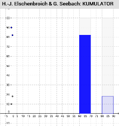
① This GeoGebra example, titled "Pipettes," demonstrates an interactive geometric simulation that visualizes concepts from hypothesis testing, rational numbers, vectors, integral calculus, and squares, likely modeling liquid transfer or data distribution in a statistical context. ② Core mathematical concepts include hypothesis testing, rational numbers, vectors, definite integrals, and square geometry, blending statistical inference with calculus and geometric visualization. ③ Construction highlights: Based on the summary, the example uses GeoGebra commands such as Sequence, Textfield, Polygon, Midpoint, CircleArc, Point, Vector, Circle, LaTeX, First, PolyLine, Element, Segment, and If, with numerous objects (p_B, B, A, p_A, L_{vB}, ST, ET, dt, n, L_T, L_{TvBG}, Iteration, L_B, L_{TBG}, L_{vC}, L_C, L_{vA}, L_A, vc, vb, va, c, b, a, L_{maxiy}, maxy, C) and interactive controls (buttons Schaltfläche1-5, input field Eing), using iteration and vector operations to build dynamic graphics. ④ Suitable for high school to university-level mathematics education, particularly for exploring statistical inference, vector calculus, and geometric construction, and useful for teachers demonstrating the geometric meaning of hypothesis testing or for students engaging in interactive mathematical modeling.
GeoGebra Commands & Parameters
Sequence((Element[L_T, i + 1], Element[L_{vB}, i + 1]), i, 0, n - 1) → L_{TvBG}Sequence((Element[L_T, i + 1], Element[L_B, i + 1]), i, 0, n) → L_{TBG}Textfield(ST) → TxtSTTextfield(ET) → TxtETTextfield(SA) → TxtSATextfield(SB) → TxtSBTextfield(SC) → TxtSCTextfield(vA) → TxtvATextfield(vB) → TxtvBTextfield(vC) → TxtvCPolygon(E, F, 4) → Contain_A, k, l, m, p_4, G, HMidpoint(m) → IMidpoint(p_4) → JMidpoint(I, G) → KMidpoint(J, E) → LCircleArc(H, K, L) → b_APoint(b_A) → MVector(M, K) → v_APoint(b_A) → NCircle(N, O) → k_APolygon(E_1, F_1, 4) → Contain_B, k_1, l_1, m_1, p_1, G_1, H_1Midpoint(m_1) → I_1Midpoint(p_1) → J_1Midpoint(I_1, G_1) → K_1Midpoint(J_1, E_1) → L_1CircleArc(H_1, K_1, L_1) → b_BPoint(b_B) → M_1Vector(M_1, K_1) → v_BPoint(b_B) → N_1Circle(N_1, O_1) → k_BPolygon(E_2, F_2, 4) → Contain_C, k_2, l_2, m_2, p_2, G_2, H_2Midpoint(m_2) → I_2Midpoint(p_2) → J_2Midpoint(I_2, G_2) → K_2Midpoint(J_2, E_2) → L_2CircleArc(H_2, K_2, L_2) → b_CPoint(b_C) → M_2Vector(M_2, K_2) → v_CPoint(b_C) → N_2Circle(N_2, O_2) → k_CLaTeX(vA, false, false) → TextvALaTeX(vB, false, false) → TextvBLaTeX(vC, false, false) → TextvCFirst(Sequence[(Element[L_T, i + 1], Element[L_A, i + 1]), i, 0, n + 1], Iteration + 1) → L_{TAE}PolyLine(L_{TAE}) → Str_{AE}First(L_{TBG}, Iteration + 1) → L_{TBE}PolyLine(L_{TBE}) → Str_{BE}PolyLine(L_{TCE}) → Str_{CE}Element(L_A, Iteration + 1) → Bestand_AElement(L_B, Iteration + 1) → Bestand_BElement(L_C, Iteration + 1) → Bestand_CElement(L_{vA}, Iteration) → Aenderung_AElement(L_{vB}, Iteration) → Aenderung_BElement(L_{vC}, Iteration) → Aenderung_CFirst(Sequence[(Element[L_T, i + 1], Element[L_{vA}, i + 1]), i, 0, n], Iteration) → L_{TvAE}PolyLine(L_{TvAE}) → Str_{vAE}First(L_{TvBG}, Iteration) → L_{TvBE}PolyLine(L_{TvBE}) → Str_{vBE}PolyLine(L_{TvCE}) → Str_{vCE}Element(L_{TCE}, Iteration) → DrAElement(L_{TCE}, Iteration + 1) → DrCPolygon(DrA, DrB, DrC) → Dreieck_C, dr3, dr2, dr1Element(L_{TvCE}, Iteration) → vCESegment(TX, vCE) → Strecke_{vC}Sequence((Element[L_T, i + 1], Element[L_A, i + 1]), i, 0, n) → L_{TAG}Sequence((Element[L_T, i + 1], Element[L_{vA}, i + 1]), i, 0, n - 1) → L_{TvAG}If(b, 1, 5) → dPolyLine(L_{TAG}) → Str_{AG}PolyLine(L_{TvAG}) → Str_{vAG}PolyLine(L_{TBG}) → Str_{BG}PolyLine(L_{TvBG}) → Str_{vBG}PolyLine(L_{TCG}) → Str_{CG}PolyLine(L_{TvCG}) → Str_{vCG}Polygon(R1, R2, P, D) → Vieleck1, r1, r2, p, d_1Polygon(R3, R4, R, Q) → Vieleck2, r3, r4, r, qPolygon(R1, R2, U, S) → Vieleck3, r1_1, r2_1, u, sPolygon(R3, R4, W, V) → Vieleck4, r3_1, r4_1, w, v
AI Drawing Prompt Reference
Draw a geometric simulation with three side-by-side containers, each consisting of a square frame and an inner circular arc with a movable point on it, from which a vector points to an arc endpoint. Label the containers A, B, and C, each with a vector label and numeric input field. Below the containers, draw two polyline paths formed by sequences of points: one showing a time-varying trajectory and the other a cumulative path, with their visible length controlled by an iteration count. The overall figure illustrates hypothesis testing, vectors, and integral concepts, including interactive buttons and text input areas.
The prompt above was compiled from the original drawing commands and is for reference only.