
Logistic Growth Model Interactive Demo (1)
Loading the math board and drawing, please wait…
In collections
ICME 13, TSG 46: Growth and Modelling with KUMULATOR
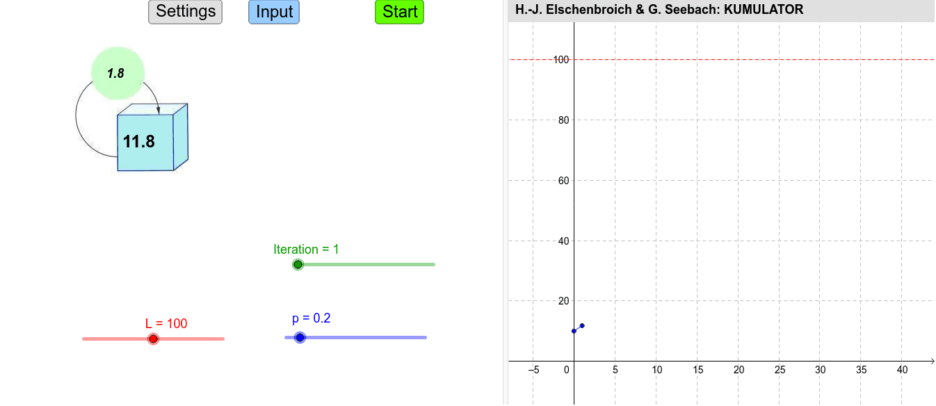
① This GeoGebra example dynamically illustrates the logistic growth curve, showing the S-shaped increase of a population or quantity under limited resources. ② Core mathematical concepts include the logistic equation, numerical solutions of differential equations, iteration, limits and asymptotes, and the influence of parameters on growth rate and carrying capacity. ③ Construction highlights: interactive controls such as Textfield, LaTeX, and Sliders adjust parameters (e.g., growth rate r, initial value, carrying capacity K); Sequence and Iteration generate iterative sequences; PolyLine, Segment, and Polygon draw curves and auxiliary shapes; buttons (Schaltfläche) control animation and reset. ④ Suitable for high school to university level mathematics or mathematical biology, useful for teaching population growth models, numerical methods for differential equations, and parameter sensitivity analysis.
GeoGebra Commands & Parameters
Textfield(ST) → TxtSTTextfield(ET) → TxtETTextfield(SA) → TxtSATextfield(SB) → TxtSBTextfield(SC) → TxtSCTextfield(vA) → TxtvATextfield(vB) → TxtvBTextfield(vC) → TxtvCLaTeX(vA, false, false) → TextvALaTeX(vB, false, false) → TextvBLaTeX(vC, false, false) → TextvCFirst(Sequence[(Element[L_T, i + 1], Element[L_A, i + 1]), i, 0, n + 1], Iteration + 1) → L_{TAE}PolyLine(L_{TAE}) → Str_{AE}PolyLine(L_{TBE}) → Str_{BE}PolyLine(L_{TCE}) → Str_{CE}Element(L_A, Iteration + 1) → Bestand_AElement(L_B, Iteration + 1) → Bestand_BElement(L_C, Iteration + 1) → Bestand_CElement(L_{vA}, Iteration) → Aenderung_AElement(L_{vB}, Iteration) → Aenderung_BElement(L_{vC}, Iteration) → Aenderung_CFirst(Sequence[(Element[L_T, i + 1], Element[L_{vA}, i + 1]), i, 0, n], Iteration) → L_{TvAE}PolyLine(L_{TvAE}) → Str_{vAE}PolyLine(L_{TvBE}) → Str_{vBE}PolyLine(L_{TvCE}) → Str_{vCE}Element(L_{TCE}, Iteration) → DrAElement(L_{TCE}, Iteration + 1) → DrCPolygon(DrA, DrB, DrC) → Dreieck_C, dr3, dr2, dr1Element(L_{TvCE}, Iteration) → vCESegment(TX, vCE) → Strecke_{vC}Sequence((Element[L_T, i + 1], Element[L_A, i + 1]), i, 0, n) → L_{TAG}Sequence((Element[L_T, i + 1], Element[L_{vA}, i + 1]), i, 0, n - 1) → L_{TvAG}If(b, 1, 5) → dPolyLine(L_{TAG}) → Str_{AG}PolyLine(L_{TvAG}) → Str_{vAG}PolyLine(L_{TBG}) → Str_{BG}PolyLine(L_{TvBG}) → Str_{vBG}PolyLine(L_{TCG}) → Str_{CG}PolyLine(L_{TvCG}) → Str_{vCG}
AI Drawing Prompt Reference
Create an interactive logistic growth model demo. Show three S-shaped growth curves on a time-versus-population plot, each approaching a different carrying capacity. Label each curve with its initial value, growth rate, and carrying capacity. Below or overlaid, display three rate-of-change curves for the population over time, marking the current iteration's rate point. Use a triangle to highlight the relationship between the current population and its rate of change, with a segment connecting the point to the rate curve. Include text fields and sliders to adjust parameters, plus buttons for animation and reset.
The prompt above was compiled from the original drawing commands and is for reference only.