
Epidemic Spread Model
Loading the math board and drawing, please wait…
In collections
ICME 13, TSG 46: Growth and Modelling with KUMULATOR
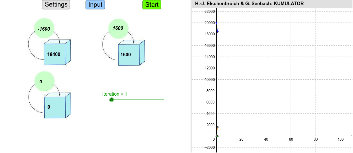
This example demonstrates the dynamics and trends of epidemic spread within a specific area. It involves core mathematical concepts such as quadratic equations, standard deviation, secant lines, random experiments, and linear equations. Key GeoGebra commands and objects used in the construction include Sequence, Textfield, LaTeX, First, PolyLine, Element, Polygon, Segment, and If. It is suitable for high school and above learners to understand the mathematical principles and visual representation in epidemic models.
GeoGebra Commands & Parameters
Sequence((Element[L_T, i + 1], Element[L_{vC}, i + 1]), i, 0, n - 1) → L_{TvCG}Sequence((Element[L_T, i + 1], Element[L_C, i + 1]), i, 0, n) → L_{TCG}Sequence((Element[L_T, i + 1], Element[L_{vB}, i + 1]), i, 0, n - 1) → L_{TvBG}Sequence((Element[L_T, i + 1], Element[L_B, i + 1]), i, 0, n) → L_{TBG}Textfield(ST) → TxtSTTextfield(ET) → TxtETTextfield(SA) → TxtSATextfield(SB) → TxtSBTextfield(SC) → TxtSCTextfield(vA) → TxtvATextfield(vB) → TxtvBTextfield(vC) → TxtvCLaTeX(vA, false, false) → TextvALaTeX(vB, false, false) → TextvBLaTeX(vC, false, false) → TextvCFirst(Sequence[(Element[L_T, i + 1], Element[L_A, i + 1]), i, 0, n + 1], Iteration + 1) → L_{TAE}PolyLine(L_{TAE}) → Str_{AE}First(L_{TBG}, Iteration + 1) → L_{TBE}PolyLine(L_{TBE}) → Str_{BE}First(L_{TCG}, Iteration + 1) → L_{TCE}PolyLine(L_{TCE}) → Str_{CE}Element(L_A, Iteration + 1) → Bestand_AElement(L_B, Iteration + 1) → Bestand_BElement(L_C, Iteration + 1) → Bestand_CElement(L_{vA}, Iteration) → Aenderung_AElement(L_{vB}, Iteration) → Aenderung_BElement(L_{vC}, Iteration) → Aenderung_CFirst(Sequence[(Element[L_T, i + 1], Element[L_{vA}, i + 1]), i, 0, n], Iteration) → L_{TvAE}PolyLine(L_{TvAE}) → Str_{vAE}First(L_{TvBG}, Iteration) → L_{TvBE}PolyLine(L_{TvBE}) → Str_{vBE}First(L_{TvCG}, Iteration) → L_{TvCE}PolyLine(L_{TvCE}) → Str_{vCE}Element(L_{TCE}, Iteration) → DrAElement(L_{TCE}, Iteration + 1) → DrCPolygon(DrA, DrB, DrC) → Dreieck_C, dr3, dr2, dr1Element(L_{TvCE}, Iteration) → vCESegment(TX, vCE) → Strecke_{vC}Sequence((Element[L_T, i + 1], Element[L_A, i + 1]), i, 0, n) → L_{TAG}Sequence((Element[L_T, i + 1], Element[L_{vA}, i + 1]), i, 0, n - 1) → L_{TvAG}If(b, 1, 5) → dPolyLine(L_{TAG}) → Str_{AG}PolyLine(L_{TvAG}) → Str_{vAG}PolyLine(L_{TBG}) → Str_{BG}PolyLine(L_{TvBG}) → Str_{vBG}PolyLine(L_{TCG}) → Str_{CG}PolyLine(L_{TvCG}) → Str_{vCG}
AI Drawing Prompt Reference
Visualize the dynamics and trends of epidemic spread in a specific area, incorporating mathematical concepts like quadratic equations, standard deviation, secant lines, random experiments, and linear equations. Use distinct colored lines to show the population changes of different groups and triangles to represent key data points, forming a mathematical model of epidemic spread.
The prompt above was compiled from the original drawing commands and is for reference only.