
Physics Problem: Separable Differential Equations
Loading the math board and drawing, please wait…
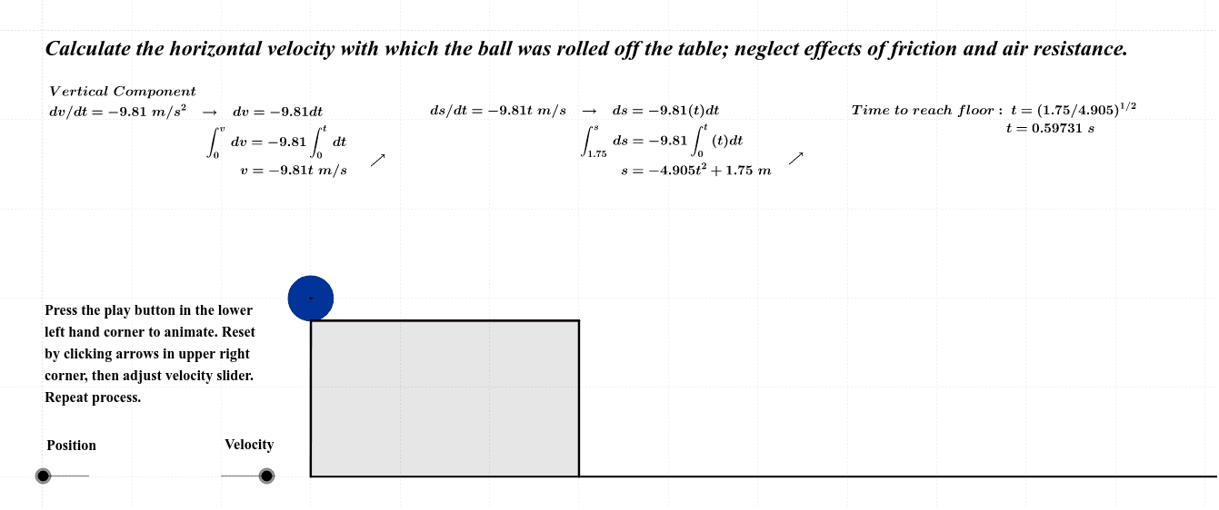
This example demonstrates a physics problem using separable differential equations. Key mathematical concepts include differential equations and separable equations. It uses commands like Intersect, Point, Segment, Polygon, Circle, OrthogonalLine, and Vector in GeoGebra. Suitable for high school physics and mathematics courses.
GeoGebra Commands & Parameters
Intersect(xAxis, yAxis) → APoint(yAxis) → BSegment((5, 0), (5, 2)) → gSegment((0, 0), (0, 2)) → fSegment(B, D) → a_2Polygon(A, B, D, E) → poly1, a_1, b_2, d, eIntersect(p, c, (11.32455531795991, 1.5032515232604737E-9)) → CIntersect(p, c, (11.32455531795991, 1.5032515232604737E-9)) → FIntersect(i, j) → GIntersect(i, k) → HSegment(H, G) → lIntersect(p, m, (10.916079783099388, 0.250000000000135)) → IIntersect(k, m) → JSegment(J, I) → nIntersect(m, g) → KSegment(K, I) → qIntersect(h, r, (2, 1.75)) → LIntersect(p, r, (7.1713, 1.7642728155)) → MCircle(M, 0.25) → tPoint(Circle[(0, 1.75), 5]) → NSegment(K, I) → b_1Segment(E, O) → d_1Intersect(r, a_2) → QCircle(Q, 0.25) → c_1Circle(Q, 0.26867087944031054) → g_1OrthogonalLine(M, d_1) → h_1Intersect(h_1, d_1) → RSegment(R, M) → i_1OrthogonalLine(C, xAxis) → j_1OrthogonalLine(I, j_1) → k_1OrthogonalLine(I, xAxis) → l_1Intersect(c, l_1) → SSegment(S, I) → m_1Segment((5, 2), (a, 2)) → n_1Intersect(r, n_1) → TCircle(T, 0.25) → q_1Circle(T, 0.23573262929063565) → r_1Vector((5, 2), (a, 2)) → u_1Vector((a, 2), (a, 0.25)) → v_1Vector((5, 2), (a, 0.25)) → w_1Point(u_3) → USegment(U, T) → u_2Segment(U, M) → w_2Segment(T, M) → vSegment((2, 1.75), N) → s_1Segment(P, V) → bPolygon(P, N, E, V) → poly2, p_1, n_2, e_1, v_2OrthogonalLine(M, f_1) → c_2Intersect(f_1, c_2) → WCircle(W, 0.25) → d_2Circle(W, 0.23702296356931926) → e_2Point(Circle[(2, 0), 12]) → ZSegment((2, 0), Z) → f_2Segment(D, M) → wSegment(D, T) → t_1Segment(D, T) → g_2OrthogonalLine(M, d_1) → h_2Intersect(h_2, d_1) → A_1Segment(A_1, M) → i_2Point(Circle[(5, 2), i_2]) → B_1Segment((5, 2), B_1) → u
AI Drawing Prompt Reference
Draw a coordinate system with x and y axes. Mark the intersection point. Draw a horizontal line segment from (5,0) to (5,2) and a vertical line segment from (0,0) to (0,2). Connect these segments and another point on the y-axis to form a quadrilateral. Inside the quadrilateral, draw a circle centered at (7.1713, 1.7642728155) with a radius of 0.25. Mark several points on the circle and connect them to form a closed shape. Finally, draw perpendicular lines from the circle's center to the x-axis and y-axis, mark the intersection points, and connect them to form new shapes.
The prompt above was compiled from the original drawing commands and is for reference only.