
Physics Problem: Separable Differential Equations by Earl Samuelson
Loading the math board and drawing, please wait…
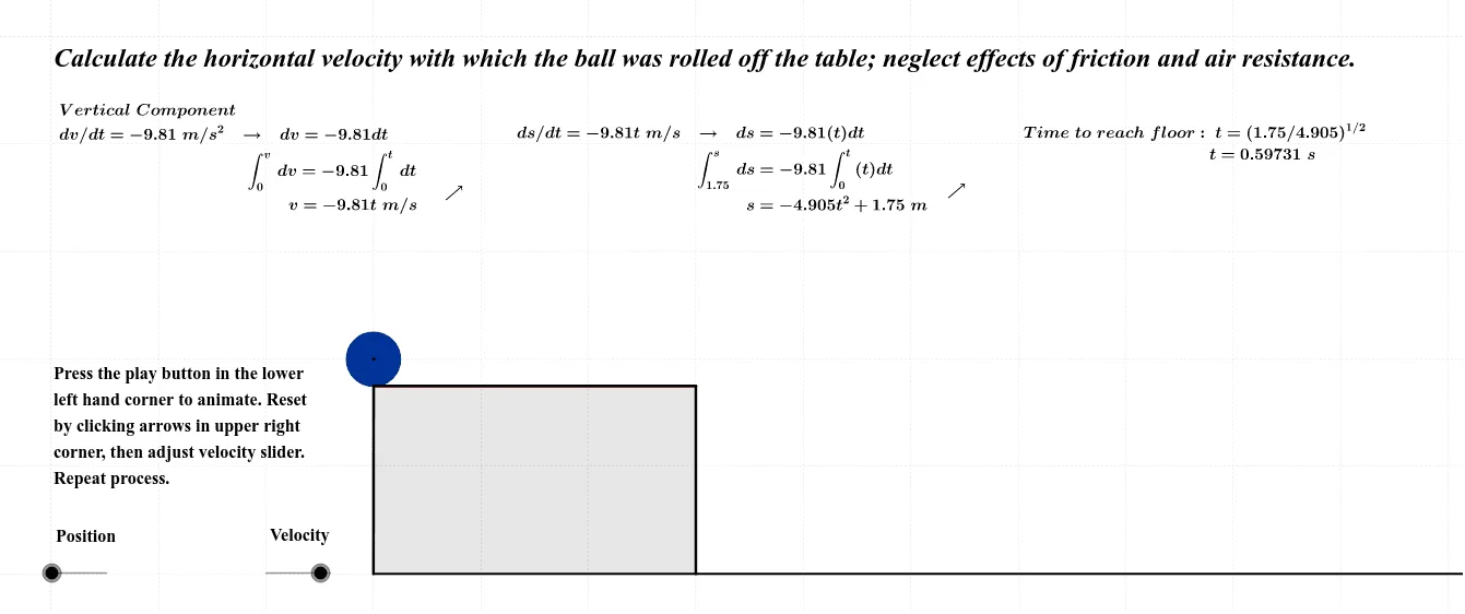
This example demonstrates how to graph the solution curves of separable differential equations using GeoGebra. It involves core mathematical concepts such as differential equations, separation of variables, function graphs, vectors, and three-dimensional space. Key GeoGebra commands and objects used in the construction include Intersect, Point, Segment, Polygon, Circle, OrthogonalLine, and Vector. Suitable for high school students and above to learn and understand the application of differential equations in physics problems, or for teaching demonstrations.
GeoGebra Commands & Parameters
Intersect(xAxis, yAxis) → APoint(yAxis) → BSegment((5, 0), (5, 2)) → gSegment((0, 0), (0, 2)) → fSegment(B, D) → a_2Polygon(A, B, D, E) → poly1, a_1, b_2, d, eIntersect(p, c, (11.32455531795991, 1.5032515232604737E-9)) → CIntersect(p, c, (11.32455531795991, 1.5032515232604737E-9)) → FIntersect(i, j) → GIntersect(i, k) → HSegment(H, G) → lIntersect(p, m, (10.916079783099388, 0.250000000000135)) → IIntersect(k, m) → JSegment(J, I) → nIntersect(m, g) → KSegment(K, I) → qIntersect(h, r, (2, 1.75)) → LIntersect(p, r, (7.1713, 1.7642728155)) → MCircle(M, 0.25) → tPoint(Circle[(0, 1.75), 5]) → NSegment(K, I) → b_1Segment(E, O) → d_1Intersect(r, a_2) → QCircle(Q, 0.25) → c_1Circle(Q, 0.26867087944031054) → g_1OrthogonalLine(M, d_1) → h_1Intersect(h_1, d_1) → RSegment(R, M) → i_1OrthogonalLine(C, xAxis) → j_1OrthogonalLine(I, j_1) → k_1OrthogonalLine(I, xAxis) → l_1Intersect(c, l_1) → SSegment(S, I) → m_1Segment((5, 2), (a, 2)) → n_1Intersect(r, n_1) → TCircle(T, 0.25) → q_1Circle(T, 0.23573262929063565) → r_1Vector((5, 2), (a, 2)) → u_1Vector((a, 2), (a, 0.25)) → v_1Vector((5, 2), (a, 0.25)) → w_1Point(u_3) → USegment(U, T) → u_2Segment(U, M) → w_2Segment(T, M) → vSegment((2, 1.75), N) → s_1Segment(P, V) → bPolygon(P, N, E, V) → poly2, p_1, n_2, e_1, v_2OrthogonalLine(M, f_1) → c_2Intersect(f_1, c_2) → WCircle(W, 0.25) → d_2Circle(W, 0.23702296356931926) → e_2Point(Circle[(2, 0), 12]) → ZSegment((2, 0), Z) → f_2Segment(D, M) → wSegment(D, T) → t_1Segment(D, T) → g_2OrthogonalLine(M, d_1) → h_2Intersect(h_2, d_1) → A_1Segment(A_1, M) → i_2Point(Circle[(5, 2), i_2]) → B_1Segment((5, 2), B_1) → u