
Physics Problem: Separable Differential Equations Visualized
Loading the math board and drawing, please wait…
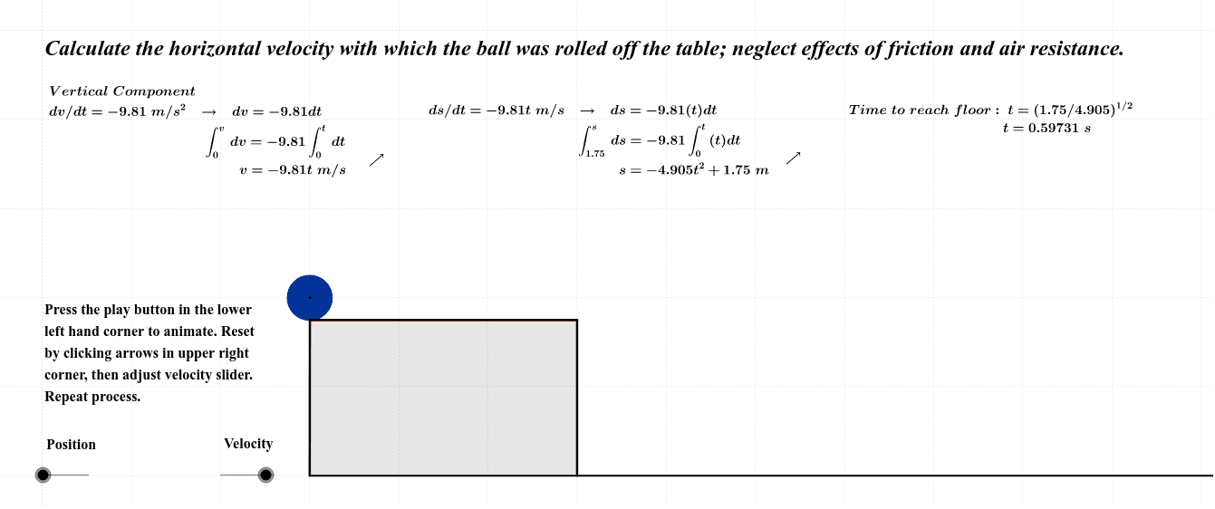
This GeoGebra example demonstrates how a physics problem involving separable differential equations can be modeled through dynamic geometry. It constructs a complex figure using points, segments, polygons, circles, perpendicular lines, and vectors, with multiple intersections and enclosed regions, to represent the behavior of solution curves or physical quantities. The core mathematical concepts include solving separable differential equations, linear regression, difference and slope, trigonometry, and properties of general quadrilaterals. The construction employs GeoGebra commands such as Intersect, Point, Segment, Polygon, Circle, OrthogonalLine, and Vector, creating objects like s, A, B, D, g, f, E, poly1, and many others in a layered geometric setup. This resource is suitable for high school to early college students, helping them connect abstract differential equations with geometric intuition. By adjusting parameters or dragging points, learners can observe how changes affect the solution curves, deepening their understanding of physical modeling and mathematical analysis.
GeoGebra Commands & Parameters
Intersect(xAxis, yAxis) → APoint(yAxis) → BSegment((5, 0), (5, 2)) → gSegment((0, 0), (0, 2)) → fSegment(B, D) → a_2Polygon(A, B, D, E) → poly1, a_1, b_2, d, eIntersect(p, c, (11.32455531795991, 1.5032515232604737E-9)) → CIntersect(p, c, (11.32455531795991, 1.5032515232604737E-9)) → FIntersect(i, j) → GIntersect(i, k) → HSegment(H, G) → lIntersect(p, m, (10.916079783099388, 0.250000000000135)) → IIntersect(k, m) → JSegment(J, I) → nIntersect(m, g) → KSegment(K, I) → qIntersect(h, r, (2, 1.75)) → LIntersect(p, r, (7.1713, 1.7642728155)) → MCircle(M, 0.25) → tPoint(Circle[(0, 1.75), 5]) → NSegment(K, I) → b_1Segment(E, O) → d_1Intersect(r, a_2) → QCircle(Q, 0.25) → c_1Circle(Q, 0.26867087944031054) → g_1OrthogonalLine(M, d_1) → h_1Intersect(h_1, d_1) → RSegment(R, M) → i_1OrthogonalLine(C, xAxis) → j_1OrthogonalLine(I, j_1) → k_1OrthogonalLine(I, xAxis) → l_1Intersect(c, l_1) → SSegment(S, I) → m_1Segment((5, 2), (a, 2)) → n_1Intersect(r, n_1) → TCircle(T, 0.25) → q_1Circle(T, 0.23573262929063565) → r_1Vector((5, 2), (a, 2)) → u_1Vector((a, 2), (a, 0.25)) → v_1Vector((5, 2), (a, 0.25)) → w_1Point(u_3) → USegment(U, T) → u_2Segment(U, M) → w_2Segment(T, M) → vSegment((2, 1.75), N) → s_1Segment(P, V) → bPolygon(P, N, E, V) → poly2, p_1, n_2, e_1, v_2OrthogonalLine(M, f_1) → c_2Intersect(f_1, c_2) → WCircle(W, 0.25) → d_2Circle(W, 0.23702296356931926) → e_2Point(Circle[(2, 0), 12]) → ZSegment((2, 0), Z) → f_2Segment(D, M) → wSegment(D, T) → t_1Segment(D, T) → g_2OrthogonalLine(M, d_1) → h_2Intersect(h_2, d_1) → A_1Segment(A_1, M) → i_2Point(Circle[(5, 2), i_2]) → B_1Segment((5, 2), B_1) → u