Phase portraits for various differential equations

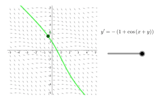
This example demonstrates how to use GeoGebra to create phase portraits for various differential equations. Phase portraits are essential tools for studying the stability and trajectories of dynamical systems, involving core mathematical concepts such as differential equations, vector fields, and trajectory analysis. Key construction points include using GeoGebra commands like If, Polygon, Sequence, and SolveODE, along with objects like n, a, A, L1, dy, ddy, ddx, poly1, L_1, numericalIntegral1, numericalIntegral2, and text1. This example is suitable for university students in mathematics, physics, or engineering, providing insights into qualitative analysis of differential equations.