
Phase Plane of a Nonlinear System: Nullclines and Slope Field
Loading the math board and drawing, please wait…
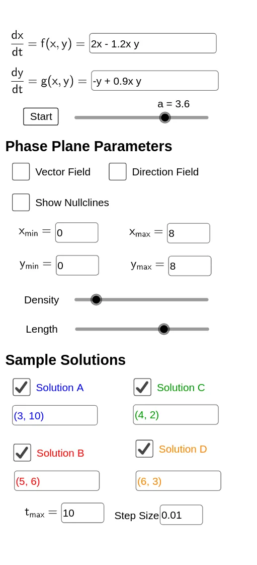
This example demonstrates the qualitative dynamics of a nonlinear differential equation system on the phase plane by combining nullclines with a slope field. It reveals how trajectories flow, how local directions are determined, and how equilibrium-related structures emerge from where the derivatives vanish. The key concepts include phase-plane analysis, nonlinear first-order ODE systems, nullclines (curves where one component of the derivative is zero), implicit curve plotting, and numerical trajectory solving. Construction-wise, it uses Textfield and multiple input objects (InputBox1–InputBox8, xmin/xmax/ymin/ymax, tmax) to set parameters and ranges; SolveODE to compute solution curves (asol, bsol, csol, dsol); SlopeField to generate the vector-field-like slope plot; and ImplicitCurve to draw the nullcline curves. Additional components such as Sequence, animation, buttons (button1, button2), layout helpers (Corner), and numerical integral readouts (numericalIntegral1/3/5/7) support iterative exploration and dynamic visualization. Suitable for advanced high school and early undergraduate study in ODEs and dynamical systems, as well as for classroom demonstrations and interactive modeling.
GeoGebra Commands & Parameters
Textfield(f) → InputBox1Textfield(xmin) → InputBox2Textfield(xmax) → InputBox3Textfield(ymin) → InputBox4Textfield(ymax) → InputBox5Textfield(delta) → InputBox6Textfield(g) → InputBox7SolveODE(g(x, y) / f(x, y), x(A), y(A), tmax, delta) → numericalIntegral1Textfield(tmax) → InputBox8SolveODE(g(x, y) / f(x, y), x(B), y(B), tmax, delta) → numericalIntegral3SolveODE(g(x, y) / f(x, y), x(C), y(C), tmax, delta) → numericalIntegral5SolveODE(g(x, y) / f(x, y), x(D), y(D), tmax, delta) → numericalIntegral7Sequence(xmin + (i * (xmax - xmin) / n), i, 1, n, 1) → l3Sequence(ymin + (i * (ymax - ymin) / n), i, 1, n, 1) → l1Sequence(Sequence[(l3(i), l1(j)), j, 1, Length[l1]], i, 1, Length[l3]) → l5Sequence(Sequence[Vector[l5(i, j), l5(i, j) + (f(l5(i, j)), g(l5(i, j)))], j, 1, Length[l1]], i, 1, Length[l3]) → l6SlopeField(g(x, y) / f(x, y), n + 1, L, xmin, ymin, xmax, ymax) → slopefield1ImplicitCurve(f(x, y)) → fnullclineImplicitCurve(g(x, y)) → gnullclineCorner(2, 1) → ETextfield(A) → InputBox9Textfield(B) → InputBox10Textfield(C) → InputBox11Textfield(D) → InputBox12
AI Drawing Prompt Reference
Create a phase-plane plot for a nonlinear first-order system by showing a slope field on the rectangle xmin to xmax and ymin to ymax, where the local direction is determined by the ratio g(x,y)/f(x,y). Overlay the two equilibrium-related nullclines as implicit curves: the curve f(x,y)=0 (the f-nullcline) and the curve g(x,y)=0 (the g-nullcline). Use the same coordinate window for all elements. Provide four adjustable initial points and numerically solve trajectories from each of them up to tmax with step delta, then display these solution curves together with the slope field and the two nullclines.
The prompt above was compiled from the original drawing commands and is for reference only.