
Parametric Curves with Trig Variations
Loading the math board and drawing, please wait…
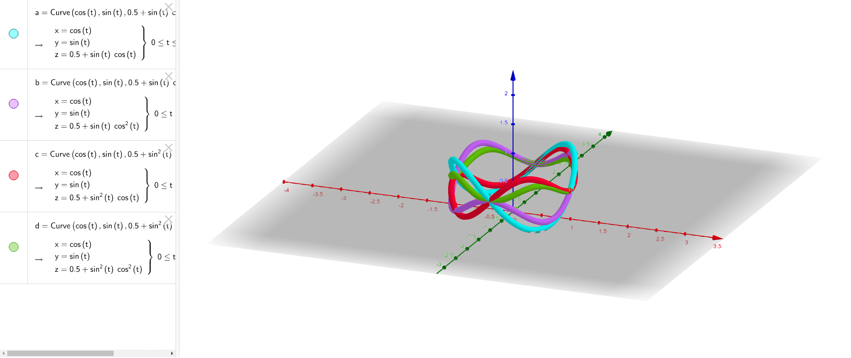
This example demonstrates the variations of parametric curves using trigonometric functions. It involves core mathematical concepts like parametric equations, trigonometry, coordinate geometry, and definite integrals. The construction uses the GeoGebra command CurveCartesian with objects a, b, c, d. Suitable for high school and above students to understand the application of parametric equations.
GeoGebra Commands & Parameters
CurveCartesian(cos(t), sin(t), 0.5 + (sin(t) * cos(t)), t, 0, (2 * π)) → aCurveCartesian(cos(t), sin(t), 0.5 + (sin(t) * cos(t)^(2)), t, 0, (2 * π)) → bCurveCartesian(cos(t), sin(t), 0.5 + (sin(t)^(2) * cos(t)), t, 0, (2 * π)) → cCurveCartesian(cos(t), sin(t), 0.5 + (sin(t)^(2) * cos(t)^(2)), t, 0, (2 * π)) → d
AI Drawing Prompt Reference
Graph four parametric curves where the x and y coordinates are cosine and sine functions, respectively, with the y coordinate also scaled by the product, square, and square product of sine and cosine, over the parameter t ranging from 0 to 2π to demonstrate variations in parametric equations involving trigonometric functions.
The prompt above was compiled from the original drawing commands and is for reference only.