
Overdamping Phenomenon
Loading the math board and drawing, please wait…
In collections
MATH1052-edX
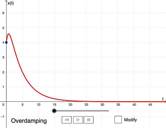
This example demonstrates the overdamping phenomenon in physical systems using differential equations and geometric graphs like straight lines and quadratic functions. Key mathematical concepts include differential equations, derivatives, and quadratic functions. Construction involves GeoGebra commands such as SolveODE, Length, and First to build dynamic models of spring-damper systems. Suitable for high school students or undergraduate students to explore the intersection of physics and mathematics.
GeoGebra Commands & Parameters
SolveODE((2 * p), ω^(2), 0, 0, x0, xprime0, maxTime, 0.04) → SolutionLength(Solution) → lenFirst(Solution, len) → LPIf(D < 0, "Underdamping", If[D ≟ 0, "Critical damping", "Overdamping"]) → textClassZip(y(P), P, LP) → LxPMax(LxP) → maxMin(LxP) → minSegment(C1, C2) → platformTextfield(x0) → Inpx0Textfield(xprime0) → Inpxprime0Textfield(m) → InpmTextfield(k) → InpkTextfield(β) → InpβRay((100, 0), (-100, 0)) → eqposIf(ylength < 0, CurveCartesian[(width * sin((((fr * 2) * π) * (t - y_1) / (y_0 - y_1)))) + x(A2), t, t, y_0, y_1], CurveCartesian[(width * sin((((fr * 2) * π) * (t - y_1) / (y_0 - y_1)))) + x(A2), t, t, y_1, y_0]) → springCurveCartesian((width * sin((((fr * 2) * π) * (t - sect) / (y_0 - sect)))) + x(A2), t, t, sect, y_0) → springFixedSegment(PS, PS + (0, sect)) → endSegment((x(A2), 0), (x(A2), 0) + (0, sect)) → endFixedIf(abs(max) < 0.4, 0.5, max) → ymaxIf(abs(min) < 0.4, -1.2, min) → yminSegment((0, ftime), ((facTime * time), ftime)) → horSegment(((facTime * time), 0), ((facTime * time), ftime)) → verTextfield(maxTime) → InpMTime
AI Drawing Prompt Reference
Draw a diagram illustrating the overdamping phenomenon in a spring-damper system. Show a displacement curve over time that decays smoothly without oscillation, derived from a differential equation. Below the curve, draw a horizontal platform line, with a spring depicted as a sine wave connecting the platform to a movable object. Include two input fields for initial displacement and velocity, and a text label indicating 'Overdamping'. Add a horizontal time axis and a vertical reference line to mark the current time. The layout should clearly connect the physical system with its mathematical representation.
The prompt above was compiled from the original drawing commands and is for reference only.