
Numerical Solutions of Equations Part 4
Loading the math board and drawing, please wait…
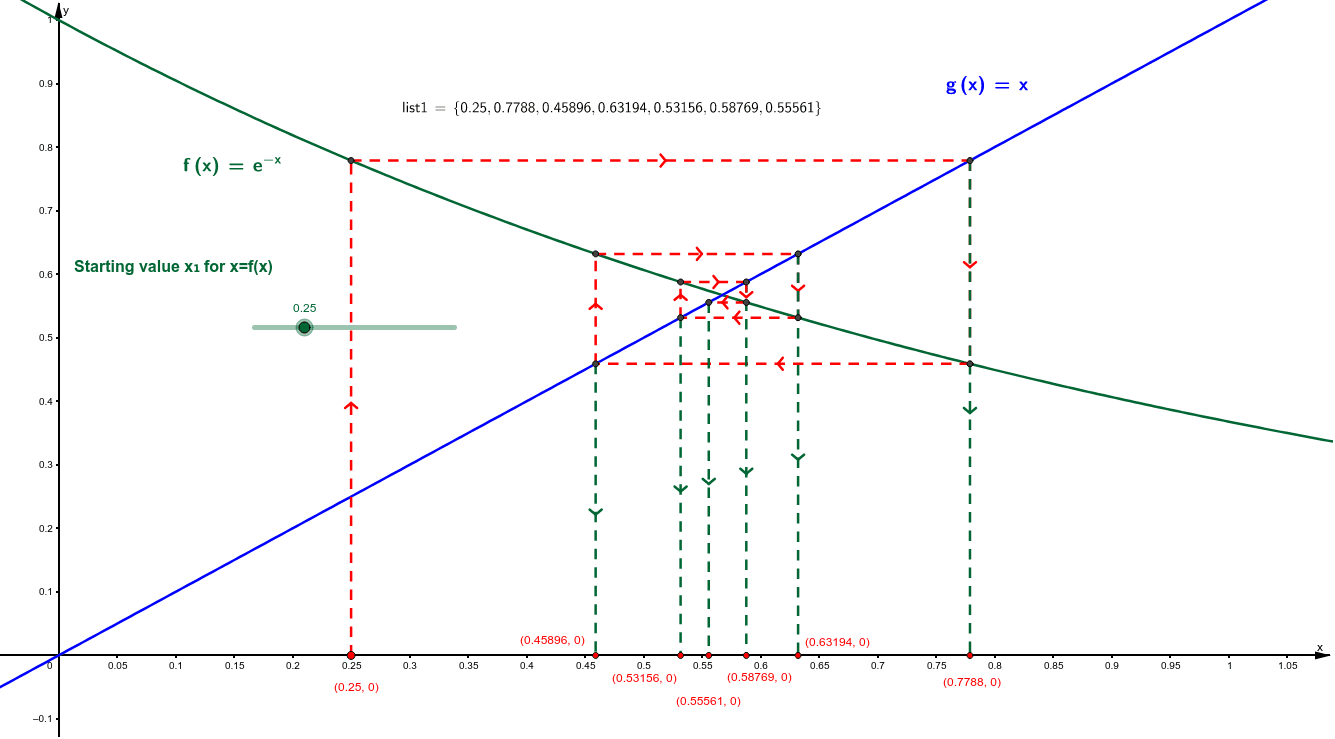
This example demonstrates numerical solutions of equations using GeoGebra, involving core math concepts like iteration, orthogonal lines, intersections, and segments. It visually shows function graphs and solution distributions through commands like LaTeX, Iteration, OrthogonalLine, Intersect, Segment, and IterationList. Suitable for high school and above, helping learners understand the geometric meaning and computational process of numerical methods.
GeoGebra Commands & Parameters
LaTeX(f, true, true) → text1LaTeX(g, true, true) → text2LaTeX(f, true, true) → text3Iteration(f, a, 6) → oOrthogonalLine(A, xAxis) → bIntersect(f, b, (0.25, 0.7788007830714049)) → BOrthogonalLine(B, b) → cIntersect(g, c) → COrthogonalLine(C, c) → dIntersect(f, d, (0.7788007830714049, 0.4589560693076638)) → DOrthogonalLine(D, d) → eIntersect(g, e) → EOrthogonalLine(E, e) → hIntersect(f, h, (0.4589560693076638, 0.6319430059834795)) → FOrthogonalLine(F, h) → iIntersect(g, i) → GOrthogonalLine(G, i) → jIntersect(f, j, (0.6319430059834795, 0.5315579766395019)) → HOrthogonalLine(H, j) → kIntersect(g, k) → ISegment(A, B) → lSegment(C, D) → nSegment(D, E) → pSegment(E, F) → qSegment(F, G) → rSegment(G, H) → sIntersect(j, xAxis) → JIntersect(h, xAxis) → KIntersect(d, xAxis) → LSegment(C, L) → a_1Segment(E, K) → b_1Segment(G, J) → c_1OrthogonalLine(I, xAxis) → d_1Intersect(d_1, xAxis) → MSegment(I, M) → e_1Intersect(f, d_1, (0.5315579766395019, 0.5876886508726961)) → NOrthogonalLine(N, d_1) → f_1Intersect(g, f_1, 1) → OOrthogonalLine(O, xAxis) → g_1Intersect(g_1, xAxis) → PSegment(I, N) → h_1Segment(N, O) → i_1Segment(O, P) → j_1Segment(B, C) → mSegment(H, I) → tIntersect(f, g_1, (0.5876886508726961, 0.5556100104627527)) → QOrthogonalLine(Q, g_1) → k_1Intersect(g, k_1, 1) → RSegment(O, Q) → l_1Segment(Q, R) → m_1OrthogonalLine(R, xAxis) → n_1Intersect(n_1, xAxis) → SSegment(R, S) → p_1Iteration(f, a, 6) → uIteration(f, a, 6) → vIterationList(f, a, 6) → list1LaTeX(list1, true, true) → text4
AI Drawing Prompt Reference
Draw the graphs of two functions, f and g, and demonstrate the numerical solution process. First, plot the graphs of f and g. Then, use iteration and orthogonal lines to find the intersection points of the functions, connecting these points sequentially to form line segments. Additionally, draw line segments orthogonal to the x-axis, marking their intersections with the functions. Finally, connect these intersection points to show the distribution of numerical solutions for the functions.
The prompt above was compiled from the original drawing commands and is for reference only.