
Number of Solutions of Simultaneous Linear Equations
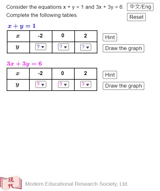
Loading the math board and drawing, please wait…
This example demonstrates the number of solutions for systems of two linear equations. It involves core math concepts like linear equations, function graphs, and the determination of solutions (no solution, one solution, infinite solutions). Construction highlights the use of GeoGebra commands and objects such as Sequence, Textfield, Line, Corner to dynamically visualize the solution sets of different equation systems. Suitable for high school mathematics teaching to understand the geometric representation and criteria for solutions of systems of equations.
GeoGebra Commands & Parameters
Sequence(Segment[(x(T_1) + (2 * k), y(T_1)), (x(T_1) + (2 * k), y(T_1) + 2)], k, 0, 4) → t_1Sequence(Segment[(x(T_1), y(T_1) + k), (x(T_1) + 8, y(T_1) + k)], k, 0, 2) → t_2Sequence(Segment[(x(T_2) + (2 * k), y(T_2)), (x(T_2) + (2 * k), y(T_2) + 2)], k, 0, 4) → t_3Sequence(Segment[(x(T_2), y(T_2) + k), (x(T_2) + 8, y(T_2) + k)], k, 0, 2) → t_4Textfield(f) → InputBox1Textfield(g) → InputBox2Line(A_1, A_2) → f_2Line(A_4, A_5) → g_2Line(A_2, A_3) → f_3Line(A_5, A_6) → g_3Corner(2, 1) → CCorner(2, 1) → Z
AI Drawing Prompt Reference
Draw a coordinate system with three parallel lines representing two linear equations, dynamically adjust parameters to observe the number of solutions for the system of equations, including no solution, one solution, and infinite solutions, using different colored line segments and text annotations to distinguish different solution sets.
The prompt above was compiled from the original drawing commands and is for reference only.