
Nullcline Plot Construction
Loading the math board and drawing, please wait…
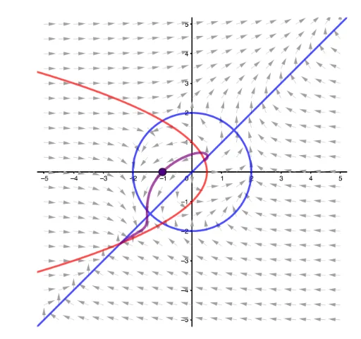
This example demonstrates how to plot nullclines for differential equations, visually representing the direction field of solutions. It involves core math concepts like differential equations, similarity transformations, sequences, and real number operations. Key GeoGebra commands and objects used include SelectedElement, ImplicitCurve, Sequence, SolveODE, and Polygon as outlined in the construction summary. Suitable for high school and above students to understand the geometric interpretation and numerical methods of differential equations.
GeoGebra Commands & Parameters
SelectedElement(L) → aSelectedElement(J) → bImplicitCurve(a) → cImplicitCurve(b) → dSequence(Sequence[Vector[(m, n), Translate[(m, n), Vector[(0.4 * (aa(m, n), bb(m, n)))]]], m, -5, 5, 0.5], n, -5, 5, 0.5) → L_1SolveODE(bb, aa, x(A), y(A), 10, 0.01) → numericalIntegral1Polygon((-5.25, -5.25), (5.25, -5.25), 4) → poly1SolveODE(bb, aa, x(A), y(A), -10, 0.01) → numericalIntegral2
AI Drawing Prompt Reference
Create a coordinate plane visualization showing nullclines and direction field for a differential equation system. First, plot two implicit curves representing the nullclines where the derivatives equal zero for each function. Then, display a direction field across a grid spanning from -5 to 5 in both x and y directions, using small arrows to indicate the slope at each point determined by the two functions. Next, from a specific point on the plane, draw one integral curve (solution curve) extending forward in time, and another integral curve extending backward in time. Finally, add a square boundary frame around the outer edges of the graphic. This visualization demonstrates the geometric interpretation and numerical methods of differential equations.
The prompt above was compiled from the original drawing commands and is for reference only.