
Normal Probability Problems Interactive Demo
Loading the math board and drawing, please wait…
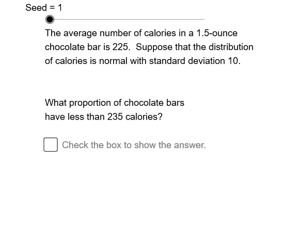
This GeoGebra example demonstrates probability calculations under the normal distribution, allowing users to dynamically adjust the mean, standard deviation, and random seed to explore Z-scores, probability intervals, and sampling distributions. Core mathematical concepts include normal distribution, standard normal distribution, Z-scores, probability density, cumulative probability, and an introduction to the central limit theorem. Construction highlights: the Normal command generates normally distributed random values, while Element, Sequence, Mod, and If build sample sequences and conditional logic. Sliders control the mean (Mn), standard deviation (StDv), and seed (Seed). Objects like ZSq1, Z1, Z2, and Z3 compute Z-scores, and DrSq1, DrSq2, etc., render distribution curves and shaded probability regions. Suitable for high school and introductory college statistics courses, this interactive tool helps visualize normal probability calculations, Z-score transformations, and random simulation in teaching.
GeoGebra Commands & Parameters
Element(StDvSq, Mod[Seed, 6] + 1) → StDvElement(MnSq, Mod[Seed, 6] + 1) → MnSequence(Mod[6 + (41 * k), 84] + 10, k, 1, 60) → OpSq01, {57, 14, 55, 12, 53, 10, 51, 92, 49, 90, 47, 88, 45, 86, 43, 84, 41, 82, 39, 80, 37, 78, 35, 76, 33, 74, 31, 72, 29, 70, 27, 68, 25, 66, 23, 64, 21, 62, 19, 60, 17, 58, 15, 56, 13, 54, 11, 52, 93, 50, 91, 48, 89, 46, 87, 44, 85, 42, 83, 40}Element(OpSq01, Seed) → OpNm01Element(DrSq1, DrNm1) → Dr1Element(ZSq1, Op04) → Z1Element(ZSq1, Op04) → Z2Mod(OpNm03, 2) → Op03Mod(OpNm02, 2) → Op02Element(VbSgSq, Op00) → VbSgElement(SbSgSq, Op00) → SbSgElement(AcSq, Op00) → AcElement(ZSq2, Op04) → Z3Element(DrSq2, DrNm2) → Dr2Element(DrSq3, DrNm3) → Dr3Element(UntSq, Op00) → UntIf(Op02 ≟ 0, QSBT1, QSBT2) → QSBT0Element(VbPlSq, Op00) → VbPlElement(SbPlSq, Op00) → SbPlIf(Op02 ≟ 0, QPBT1, QPBT2) → QPBT0Sequence(Mod[17 + (29 * k), 60] + 1, k, 1, 60) → OpSq12, {47, 16, 45, 14, 43, 12, 41, 10, 39, 8, 37, 6, 35, 4, 33, 2, 31, 60, 29, 58, 27, 56, 25, 54, 23, 52, 21, 50, 19, 48, 17, 46, 15, 44, 13, 42, 11, 40, 9, 38, 7, 36, 5, 34, 3, 32, 1, 30, 59, 28, 57, 26, 55, 24, 53, 22, 51, 20, 49, 18}Element(OpSq12, Seed) → OpNm12If(Op02 ≟ 0, "probability", "proportion") → PBNormal(Mn, StDv, SgVl) → Pr1Element(IESq2, DrNm2) → IE2Element(IESq3, DrNm3) → IE3Normal(Mn, StDv, RtVl) → Pr4Normal(Mn, StDv, LfVl) → Pr3Element(AnSq, DrNm1) → An0Element(IESq1, DrNm1) → IE1Element(DDSq, Mod[Seed, 6] + 1) → DD0If(Op03 ≟ 0, QPBT0, QPOD) → QD0If(Op03 ≟ 0, QSBT0, QSOD) → QS0If(Op02 ≟ 0, QS0, QD0) → Qs0If(Op02 ≟ 0, AnBT1, AnBT2) → AnBT0If(Op03 ≟ 0, AnBT0, An0) → Ans
AI Drawing Prompt Reference
Create an interactive normal distribution probability demo with sliders for mean, standard deviation, and random seed; draw the normal density curve and dynamically shade the probability region for a chosen interval based on the slider values; compute and display the corresponding Z‑scores, cumulative probabilities, and a schematic sampling distribution; use conditional logic to switch between probability and proportion problem types and update the annotation text accordingly.
The prompt above was compiled from the original drawing commands and is for reference only.