Normal Distribution and Standard Deviation: Visualizing Spread with Random Sampl

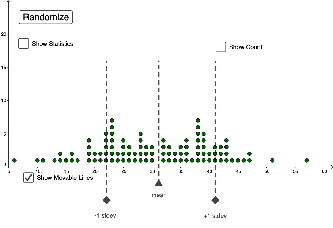
This example demonstrates how a randomly generated sample can be visualized with a dot plot to build an intuitive understanding of the normal distribution and how the standard deviation controls the data’s spread. It centers on the Normal Distribution, the meaning of stdev as a measure of dispersion around the mean (mean), and statistical counting via CountIf to estimate how many samples fall into selected intervals. The construction uses GeoGebra commands to generate data (Random) with specified parameters (mean and stdev), then plots the sample points using DotPlot. Interval statistics are computed with CountIf, supported by segment/interval boundary objects (e.g., Segment and multiple interval endpoints such as A2–A39 along with variables like k and l). It is well-suited for probability & statistics instruction at secondary-to-precalculus levels, and also for classroom demonstrations or early university teaching to connect distribution shape with the effect of standard deviation and to motivate interval-based ideas such as confidence intervals.