
Non-homogeneous 2nd Order Differential Equations
Loading the math board and drawing, please wait…
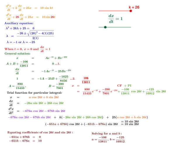
This example illustrates the graphical representation and solution of non-homogeneous second-order differential equations. It covers key concepts in calculus such as derivatives and integrals. Using GeoGebra commands like Intersect and FractionText, it dynamically shows the solutions. Suitable for university mathematics and related fields.
GeoGebra Commands & Parameters
Intersect(eq3, eq4) → DFractionText(j) → text29Intersect(eq6, eq7) → FFractionText(s) → text38FractionText(o) → text37FractionText(i) → text28FractionText(l) → text34Root(f) → A_1, B_1Intersect(eq1, eq5) → EFractionText(n) → text36Intersect(eq1, eq2) → CFractionText(B) → text8FractionText(A) → text7FractionText(p) → text20FractionText(m) → text35Intersect(eq5, eq8) → GFractionText(u) → text39
AI Drawing Prompt Reference
Draw a graphical representation of a non-homogeneous second-order differential equation. Start by plotting two curves that intersect at a point, and mark that intersection. Then plot another pair of curves, marking their intersection as well. Next, draw a function curve that crosses the horizontal axis at two points, and label both roots. After that, plot several more pairs of curves, marking each intersection point. Finally, add multiple fraction text labels near the relevant intersections or curves to indicate solution values. The overall layout should clearly show the intersections and fractional annotations.
The prompt above was compiled from the original drawing commands and is for reference only.