
Net of a Cone – Dynamic 3D to 2D Unfolding
Loading the math board and drawing, please wait…
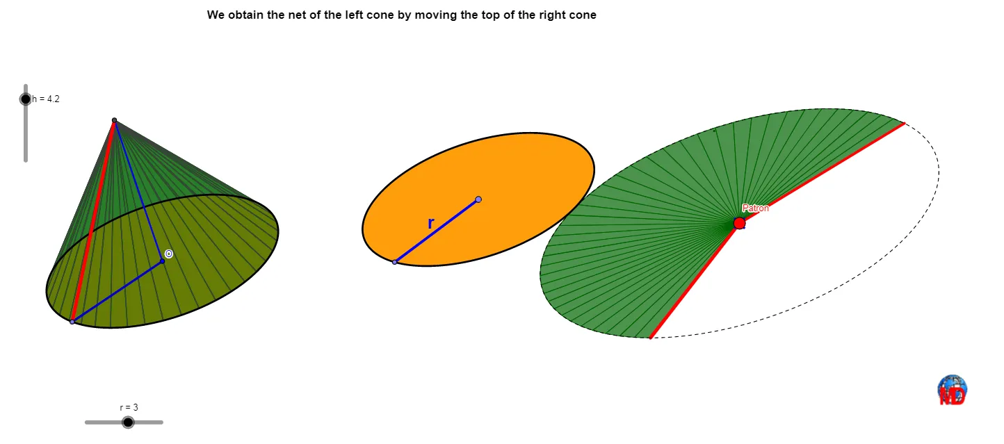
① This GeoGebra example dynamically demonstrates how a 3D cone unfolds into its 2D net (a sector), making the relationship between the solid and its flat pattern visually clear. ② Core mathematical concepts include the cone's geometry (base circle, slant height, height), the net's sector radius equal to the slant height, arc length equal to the base circumference, and the use of rotation, sequences, and parametric curves for animation. ③ Construction highlights: using commands such as Vector, Segment, Point, CurveCartesian, Intersect, Sequence, Midpoint, and Polygon to build the 3D cone and its unfolding; sliders (rap, gene, ang) control the unfolding angle and animation speed, enabling a smooth transition from solid to plane. ④ Suitable for middle or high school geometry and solid geometry classes, this resource helps students derive the cone's surface area formula, and serves as an interactive tool for teacher demonstrations or student exploration.
GeoGebra Commands & Parameters
Vector(C, X) → uVector(C, Y) → vVector(C, Z) → wSegment(B, F) → dPoint(d) → DCurveCartesian(x(F + (((gene2 + r) / rap * cos(i)) * u) + (((gene2 + r) / rap * sin(i)) * v)), y(F + (((gene2 + r) / rap * cos(i)) * u) + (((gene2 + r) / rap * sin(i)) * v)), i, 0, 6.28319) → iCurveCartesian(x(F + ((gene2 * cos(i)) * u) + ((gene2 * sin(i)) * v)), y(F + ((gene2 * cos(i)) * u) + ((gene2 * sin(i)) * v)), i, 0, 6.28319) → cPoint(c) → ECurveCartesian(x(O + ((r * cos(i)) * u) + ((r * sin(i)) * v)), y(O + ((r * cos(i)) * u) + ((r * sin(i)) * v)), i, 0, 6.28319) → bPoint(b) → ISegment(O, I) → gIntersect(xAxis, yAxis) → O_1Sequence(O + ((r * cos(i)) * u) + ((r * sin(i)) * v), i, 0, 6.28319, 0.15707963267948966) → liste1Segment(A, O) → aSequence(F + ((gene2 * cos(i)) * u) + ((gene2 * sin(i)) * v), i, 0, ((2 * π) * ang2), ((2 * π) * ang2 / 40)) → liste3Sequence(Polygon[Element[liste1, i], Element[liste1, i + 1], A], i, 0, Length[liste1]) → liste2Sequence(Polygon[Element[liste3, i], Element[liste3, i + 1], D], i, 0, Length[liste3]) → liste4Segment(D, E) → ePoint(i) → HVector(D, H) → zCurveCartesian(x(H + ((r * cos(i)) * u) + ((r * sin(i)) * v)), y(H + ((r * cos(i)) * u) + ((r * sin(i)) * v)), i, 0, 6.28319) → fCurveCartesian(x(H + ((r * cos(i)) * u) + ((r * sin(i)) * v)), y(H + ((r * cos(i)) * u) + ((r * sin(i)) * v)), i, 0, 6.28319) → jCurveCartesian(x(O + ((r * cos(i)) * u) + ((r * sin(i)) * v)), y(O + ((r * cos(i)) * u) + ((r * sin(i)) * v)), i, 0, 6.28319) → kSequence(Polygon[Element[liste1, i], Element[liste1, i + 1], A], i, 0, Length[liste1]) → liste5Sequence(Polygon[Element[liste3, i], Element[liste3, i + 1], D], i, 0, Length[liste3]) → liste6Segment(A, I) → lPoint(Circle[D, Element[liste2, 1]]) → GSegment(D, G) → mSegment(D, Element[liste3, 1]) → nSegment(D, Element[liste3, Length[liste3]]) → pSegment(D, F) → sPoint(f) → JSegment(J, H) → qMidpoint(q) → KPolygon(View3D, AA, BB, CC) → poly1, view3d, aa, bb, cc
AI Drawing Prompt Reference
Draw a cone's net, including the base circle and slant height. Start by creating the base circle and apex of the cone, then use rotation to generate the side surface of the cone's net. Connect the base circle and the corresponding points in the net to form a sector. Use sliders to control the unfolding angle and animation speed, demonstrating the dynamic transformation from 3D to 2D.
The prompt above was compiled from the original drawing commands and is for reference only.