
Net of a Cone by Edward Knote
Loading the math board and drawing, please wait…
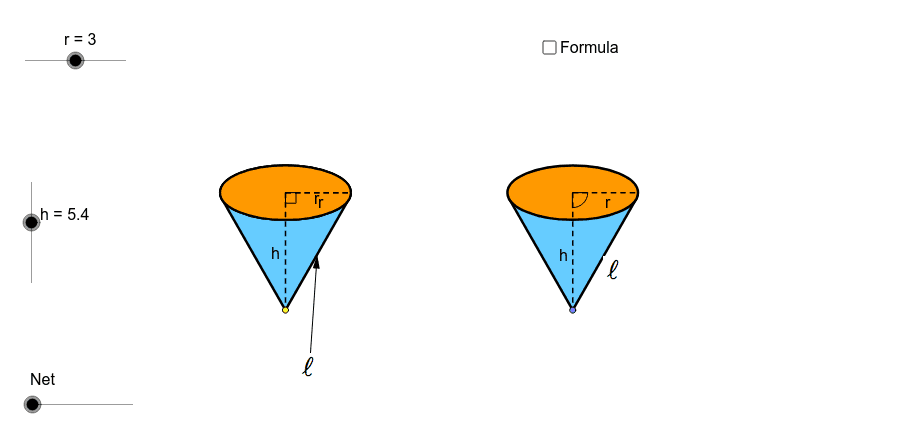
This applet demonstrates the net of a cone and its surface area formula. By adjusting the base radius and height of the cone, you can observe the changes in the shape of the cone's net. Key mathematical concepts include the geometric properties of a cone, the net, and the calculation of surface area. GeoGebra commands used include Point, Circle, Intersect, Ellipse, Vector, Translate, Arc, Segment, Angle, Line, Midpoint, If, Conic, OrthogonalLine, Tangent, Rotate, Center, Mirror, Polygon, CircleSector. Suitable for middle school and above students learning solid geometry.
GeoGebra Commands & Parameters
Point(xAxis) → ACircle(A, r) → cIntersect(c, xAxis) → B, CEllipse(E, D, C) → eIntersect(xAxis, yAxis) → FVector(F, G) → uTranslate(B, Vector[u * h]) → B'_1Translate(C, Vector[u * h]) → C'_1Translate(A, Vector[u * h]) → A'_1Translate(e, Vector[u * h]) → e'_1Arc(e'_1, C'_1, B'_1) → p_5Arc(e'_1, B'_1, C'_1) → qSegment(A'_1, A) → h_6Segment(A'_1, C'_1) → pAngle(A, A'_1, C'_1) → αLine(A, A'_1) → jIntersect(e'_1, j) → H, ICircle(I, r) → tIntersect(t, j, 2) → KCircle(K, I) → d_1Intersect(d_1, j, 2) → NVector(H, N) → vTranslate(H, Vector[v * n]) → H'_1Translate(D, Vector[u * h]) → D'Translate(E, Vector[u * h]) → E'Line(B, B'_1) → lLine(C, C'_1) → mIntersect(d_1, l, 1) → PIntersect(d_1, m, 1) → QVector(B'_1, P) → zVector(C'_1, Q) → u_1Translate(B'_1, Vector[z * n]) → B''Translate(C'_1, Vector[u_1 * n]) → C''Midpoint(B'_1, A'_1) → RMidpoint(B, A) → SLine(R, S) → a_1Intersect(q, a_1) → T,Intersect(d_1, a_1, 1) → UVector(T, U) → v_1Translate(T, Vector[v_1 * n]) → T'If(n ≟ 0.01, B'_1, If[n < 1, B'', P]) → B_1If(n ≟ 0.01, T, If[n < 1, T', U]) → D_1If(n ≟ 0.01, H, If[n < 1, H'_1, N]) → E_1If(n ≟ 0.01, C'_1, If[n < 1, C'', Q]) → F_1Conic(B_1, D_1, E_1, F_1, I) → g_1Conic(I, B_1, D_1, E_1, F_1) → h_1OrthogonalLine(I, j) → l_1OrthogonalLine(H, j) → b_2Intersect(m, l_1) → H_2Midpoint(H_2, C'_1) → I_2OrthogonalLine(C'_1, m) → i_2Segment(K, F_1) → m_4Translate(e, Vector[u * h]) → e'Tangent(A, e'_1) → a, bIntersect(e', b) → J, G_2Intersect(e', a) → L, R_2Segment(A, J) → fSegment(A, L) → gCircle(I, sqrt(h^(2) + r^(2))) → kIntersect(k, j, 1) → MCircle(M, sqrt(h^(2) + r^(2))) → sSegment(M, I) → iRotate(I, γ, M) → I'_1Rotate(I, -γ, M) → I'_2OrthogonalLine(I'_2, i_2) → b_1Intersect(b_2, b_1) → OMidpoint(H, O) → VCircle(V, O) → c_1Vector(O, I'_2) → wCenter(g_1) → WSegment(W, F_1) → e_1Vector(H, A) → w_1Translate(H, Vector[w_1 * (n - 1)]) → H'If(n < 1, H, If[n < 2, H', A]) → ZSegment(H, Z) → f_1Rotate(I, -δ, M) → I'Vector(L, I') → z_1Translate(c_1, Vector[w * (n - 2)]) → k_1Center(k_1) → A_1Intersect(k_1, j) → C_1, Q_1Rotate(C_1, 180° * (n - 2), A_1) → G_1If(n < 2, H, If[n ≤ 3, G_1, I'_2]) → H_1Mirror(H_1, j) → I_1Translate(L, Vector[z_1 * (n - 2)]) → L'If(n < 2, L, If[n ≤ 3, L', I']) → J_1Mirror(J_1, j) → K_1Conic(I_1, H_1, J_1, I, K_1) → p_1Vector(A, M) → i_1Translate(A, Vector[i_1 * (n - 2)]) → A'If(n < 2, A, If[n ≤ 3, A', M]) → L_1Tangent(L_1, p_1) → j_1, m_1Intersect(p_1, m_1, 1) → M_1Intersect(p_1, j_1, 1) → N_1Polygon(L_1, M_1, N_1) → poly1, n_1, l_2, m_2Arc(p_1, N_1, M_1) → q_1Line(L_1, b_2) → r_1Intersect(p_1, r_1, 1) → O_1Intersect(p_1, r_1, 2) → P_1Arc(p_1, P_1, O_1) → s_1Polygon(L_1, O_1, I_1) → poly2, i_3, l_3, o_1Polygon(L_1, H_1, P_1) → poly3, p_2, l_4, h_2Arc(p_1, O_1, I_1) → t_1Arc(p_1, H_1, P_1) → c_2Segment(L_1, I_1) → a_2Segment(L_1, H_1) → d_2Arc(p_1, H_1, I_1) → e_2Polygon(I_1, L_1, H_1) → poly4, h_3, i_4, l_5CircleSector(M, I'_2, I'_1) → f_2CircleSector(M, I'_2, I'_1) → g_2Arc(p_1, H_1, I_1) → k_2Segment(M_1, L_1) → j_2Segment(N_1, L_1) → n_2Polygon(I_1, L_1, H_1) → poly5, h_4, i_5, l_6Arc(p_1, H_1, I_1) → q_2Polygon(J, A, L) → poly6, l_7, j_3, a_3Point(xAxis) → R_1OrthogonalLine(R_1, xAxis) → r_2Intersect(i_2, r_2) → S_1Circle(R_1, r) → s_2Intersect(s_2, xAxis) → T_1, U_1OrthogonalLine(T_1, i_2) → t_2OrthogonalLine(V_1, i_2) → b_3OrthogonalLine(W_1, i_2) → c_3Intersect(i_2, t_2) → Z_1Intersect(i_2, b_3) → A_2Intersect(i_2, c_3) → B_2Ellipse(A_2, B_2, Z_1) → d_3Tangent(R_1, d_3) → e_3, f_3Intersect(d_3, f_3, 1) → C_2Intersect(d_3, e_3, 1) → D_2Polygon(C_2, D_2, R_1) → poly7, r_3, c_4, d_4Ellipse(A_2, B_2, Z_1) → g_3OrthogonalLine(U_1, xAxis) → k_3Intersect(g_3, k_3) → E_2, J_2Segment(S_1, E_2) → m_3Segment(S_1, R_1) → n_3Intersect(d_3, m_3, 1) → F_2Midpoint(g) → K_2Midpoint(f_1) → L_2Point(j) → M_2Midpoint(I_1, A') → N_2Midpoint(A', H_1) → O_2Vector(M_2, N_2) → u_2Vector(M_2, O_2) → v_2Line(M_2, r_1) → p_3Point(p_3) → P_2Vector(P_2, K_2) → z_2Vector(P_2, L_2) → u_3Center(g_3) → Q_2Angle(F_2, Q_2, R_1) → εSegment(I_1, H_1) → q_3Intersect(k_2, q_3, 2) → S_2Point(poly7) → T_2
AI Drawing Prompt Reference
Draw the net of a cone with adjustable base radius and height. Start by drawing a circle as the base, then draw a vertical line segment from the center as the height of the cone. Next, draw a part of an ellipse starting from the center, representing a part of the cone's side surface. Through translation and rotation, expand the elliptical part into a sector to form the cone's net. Finally, add auxiliary lines and labels to demonstrate the geometric properties of the cone and the construction process of the net.
The prompt above was compiled from the original drawing commands and is for reference only.