
Nautile Spiral
Loading the math board and drawing, please wait…
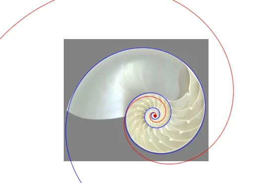
This example demonstrates the construction and properties of the Nautile spiral curve. It involves core mathematical concepts such as parametric equations, coordinate geometry, and probability & statistics (normal distribution). Key GeoGebra commands used include CurveCartesian, Angle, Distance, and Fit. Suitable for high school students and math enthusiasts learning geometric representations of parametric curves and probability distributions.
GeoGebra Commands & Parameters
CurveCartesian((r(t) * cos(t)), (r(t) * sin(t)), t, -20, 10) → aAngle((1, 0), C, A1) → B1Distance(C, A1) → C1Distance(C, A2) → C2Distance(C, A3) → C3Distance(C, A4) → C4Distance(C, A5) → C5Distance(C, A6) → C6Distance(C, A7) → C7Distance(C, A8) → C8Distance(C, A9) → C9Distance(C, A10) → C10Distance(C, A11) → C11Distance(C, A12) → C12Distance(C, A13) → C13Distance(C, A14) → C14Distance(C, A15) → C15Distance(C, A16) → C16Distance(C, A17) → C17Distance(C, A18) → C18Distance(C, A19) → C19Distance(C, A20) → C20Distance(C, A21) → C21Distance(C, A22) → C22Distance(C, A23) → C23Distance(C, A24) → C24Distance(C, A25) → C25Distance(C, A26) → C26Distance(C, A27) → C27Distance(C, A28) → C28Distance(C, A29) → C29Distance(C, A30) → C30Distance(C, A31) → C31Distance(C, A32) → C32Distance(C, A33) → C33Distance(C, A34) → C34Distance(C, A35) → C35Distance(C, A36) → C36Distance(C, A37) → C37Distance(C, A38) → C38Distance(C, A39) → C39Distance(C, A40) → C40Distance(C, A41) → C41Distance(C, A42) → C42Distance(C, A43) → C43Distance(C, A44) → C44Distance(C, A45) → C45Distance(C, A46) → C46Distance(C, A47) → C47Distance(C, A48) → C48Distance(C, A49) → C49Distance(C, A50) → C50Fit(D4:D50, {1, x}) → fCurveCartesian((ℯ^(f(t)) * cos(t)), (ℯ^(f(t)) * sin(t)), t, 8, 30) → b
AI Drawing Prompt Reference
Draw a nautilus spiral curve defined by a parametric equation where the radius is a function of the angle, with the angle ranging from -20 to 10. Place a fixed center point and mark a series of points along the curve. Measure and display the distances from the center to each of these points, and also show an angle formed by the center, a reference point, and the curve's starting point. The distances should vary progressively along the spiral, suggesting a pattern that can be fitted to a normal distribution. The illustration should clearly show the spiral's expanding coils, the center, the measurement segments, and the angle marker, combining geometric and statistical elements.
The prompt above was compiled from the original drawing commands and is for reference only.