
Modeling with Sine and Cosine Functions
Loading the math board and drawing, please wait…
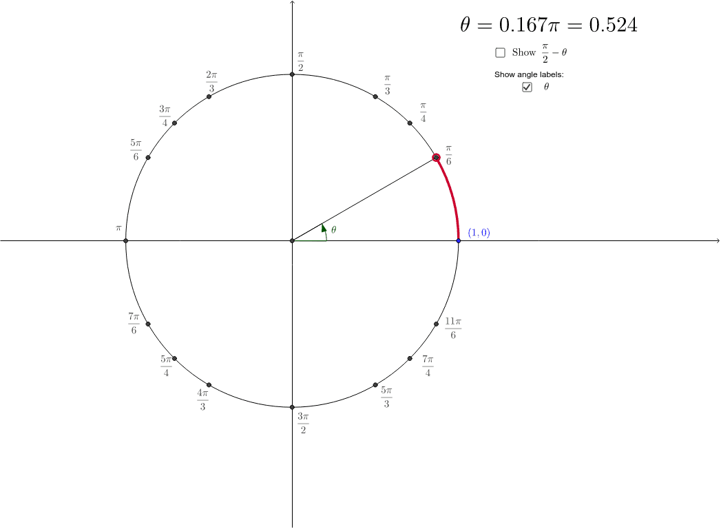
This example demonstrates periodic phenomena using sine and cosine functions. Key mathematical concepts include trigonometric functions, function graphs, and parametric equations. GeoGebra commands used include Intersect, Point, OrthogonalLine, etc. Suitable for high school math education and learning.
GeoGebra Commands & Parameters
Intersect(xAxis, yAxis) → OriginPoint(Unit) → COrthogonalLine(C, xAxis) → aIntersect(xAxis, a) → PtCosOnXSegment(C, PtCosOnX) → sineSegment(Origin, C) → rCircleSector(Origin, Pt1, C) → sectorthetaOrthogonalLine(C, r) → bCircleArc(Origin, Pt1, C) → arcthetaOrthogonalLine(C, yAxis) → cRotate(Pt1, 0.5235987755982988, Origin) → Piovr6Rotate(Pt1, 0.7853981633974483, Origin) → Piovr4Rotate(Pt1, 1.0471975511965976, Origin) → Piovr3Intersect(Unit, yAxis) → Pi3ovr2, Piovr2Rotate(Piovr2, 0.5235987755982988, Origin) → Pi2ovr3Rotate(Piovr2, 0.7853981633974483, Origin) → Pi3ovr4Rotate(Piovr2, 1.0471975511965976, Origin) → Pi5ovr6Intersect(Unit, xAxis) → Pi1, Pi02PiMirror(Pi2ovr3, xAxis) → Pi4ovr3Mirror(Pi3ovr4, xAxis) → Pi5ovr4Mirror(Pi5ovr6, xAxis) → Pi7ovr6Mirror(Piovr6, xAxis) → Pi11ovr6Mirror(Piovr4, xAxis) → Pi7ovr4Mirror(Piovr3, xAxis) → Pi5ovr3OrthogonalLine(C, yAxis) → dIntersect(yAxis, d) → PtSinOnYSegment(PtSinOnY, C) → eAngle(Pi02Pi, Origin, C) → anglethetaRotate(Piovr2, -angletheta, Origin) → Piovr2'Angle(Piovr2', Origin, Piovr2) → angleNegthetaSegment(Origin, Piovr2') → gAngle(Pi02Pi, Origin, Piovr2') → anglePiovr2minthetaOrthogonalLine(Piovr2', yAxis) → fOrthogonalLine(Piovr2', xAxis) → iIntersect(f, yAxis) → AIntersect(i, xAxis) → BSegment(A, Piovr2') → jSegment(B, Piovr2') → kAngle(Piovr2', Origin, Pi02Pi) → anglePiovr2neg