
Modeling Linear Growth (Introduction to Linear Systems)
Loading the math board and drawing, please wait…
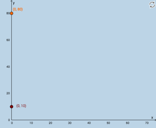
This example illustrates dynamic models of linear growth and introduces solving linear systems by graphing. It utilizes various GeoGebra commands such as constructing segments, finding intersections, and dilations. Suitable for middle school and above students to learn linear equations and functions.
GeoGebra Commands & Parameters
Textfield(f) → InputBox9Textfield(g) → InputBox10Textfield(h) → InputBox11Textfield(k) → InputBox7Textfield(e) → InputBox1Textfield(i) → InputBox2Textfield(j) → InputBox3Textfield(l) → InputBox4Textfield(r) → InputBox5Textfield(s) → InputBox6Textfield(t) → InputBox8Textfield(u) → InputBox12Intersect(f_1, f_2, 1) → CIntersect(f_1, g_1, 1) → DIntersect(f_2, g_1, 1) → EDilate(B, If[2 < v ≤ 3, 3 - v, 0], C) → B'Dilate(C, If[2 < v ≤ 4, 4 - v, 0], E) → C'Dilate(A, If[0 < v ≤ 1, 1 - v, 0], C) → A'Segment(A, A') → i_1Dilate(C, If[1 < v ≤ 2, 2 - v, 0], D) → C'_1Segment(C, C'_1) → j_1Segment(B, B') → h_1Segment(C, C') → k_1