
Mixing Two Solutions - Molarity
Loading the math board and drawing, please wait…
In collections
Chemistry2
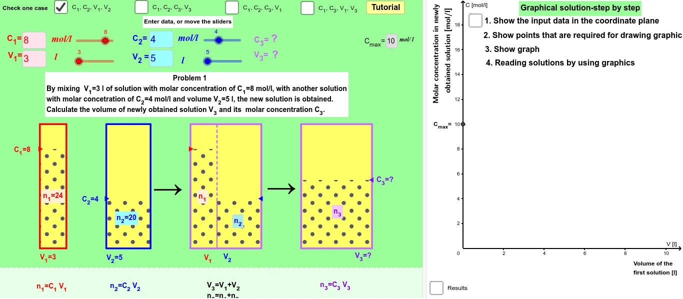
This example demonstrates the mixing of two solutions with different molar concentrations. Key mathematical concepts include the calculation of molar concentration and the changes after mixing. GeoGebra commands such as OrthogonalLine, Segment, Textfield are used for geometric construction. Suitable for high school chemistry and mathematics courses.
GeoGebra Commands & Parameters
OrthogonalLine(G_2, e) → qSegment(A_2, C_5) → g_6Textfield(V_{11}) → inputBoxV11Textfield(C_{11}) → inputBoxC11Textfield(V_{21}) → inputBoxV21Textfield(C_{21}) → inputBoxC21Textfield(C_{13}) → inputBoxC13Textfield(C_{23}) → inputBoxC23Textfield(C_{33}) → inputBoxC33Textfield(V_{13}) → inputBoxV13Textfield(C_{14}) → inputBoxC14Textfield(C_{34}) → inputBoxC34Textfield(V_{14}) → inputBoxV14Textfield(V_{34}) → inputBoxV34Line(A_3, B_3) → fLine(A_1, C_6) → bIntersect(a, b) → B_1Sequence(k, k, 0, (2 * maxv), 1) → list1OrthogonalLine(F_3, e) → gIntersect(g, f) → C_7Line(A_2, C_5) → pIntersect(q, g_6) → B_2KeepIf(0 < x ≤ 1, list2) → list3Element(list3, 1) → elemIndexOf(elem, list2) → indexElement(list1, index) → scaleLine(B_4, C_4) → iIntersect(e, i) → A_4Segment(E_1, C_6) → b_1Segment(C_6, F_1) → c_1Segment(D_1, B_1) → a_1Segment(B_1, G_1) → d_1Segment(A_1, C_6) → g_5Segment(G_2, B_2) → d_2Segment(B_2, D_2) → a_2Segment(C_5, E_2) → b_2Line(A_3, B_3) → cSegment(C_5, F_2) → c_2Segment(G_3, B_3) → d_3Segment(D_3, B_3) → a_3Segment(E_3, C_7) → b_3Segment(C_7, F_3) → c_3Segment(G_4, B_4) → d_4Segment(B_4, D_4) → a_4Segment(F_4, C_4) → c_4Segment(C_4, E_4) → b_4Segment(A_4, C_4) → g_4Midpoint(D_2, E_2) → S_2Midpoint(D_3, E_3) → S_3Midpoint(D_4, E_4) → S_4Midpoint(D_1, E_1) → S_1VerticalText(Oy) → OyvSegment(A_3, C_7) → g_7Ray(F_3, C_7) → hMin(C_{13}, C_{23}) → min3Max(C_{13}, C_{23}) → max3VerticalText(Oy2) → text3Polygon(H_1, H_2, I_2, I_1) → polyz1, h_1, i_1, j_1, k_5Polygon(H_3, H_4, I_4, I_3) → poly1z2, n_1, o_1, p_5, q_5Polygon(H_8, H_9, I_9, I_8) → poly1z3, u_5, v_1, w_1, x_1Polygon(H_1, H_2, J_2, J_1) → poly1t1, h_2, i_2, m_1, l_1Polygon(H_3, H_4, J_4, J_3) → poly1t2, n_2, o_2, t_5, r_5Polygon(H_8, H_9, J_9, J_8) → poly1t3, u_6, v_2, z_1, y_1Polygon(H_5, H_7, I_7, I_5) → poly1, h_5, h_7, i_7, i_5Polygon(H_5, H_6, J_6, J_5) → poly2, h_3, h_6, j_6, j_5Polygon(H_6, H_7, J_7, J'_6) → poly3, h_4, h_8, j_7, j'_6Segment(H_6, I_6) → dTextfield(C_{12}) → inputBoxC12Textfield(C_{22}) → inputBoxC22Textfield(C_{32}) → inputBoxC32Textfield(V_{32}) → inputBoxV32Textfield(maxc) → inputBox1
AI Drawing Prompt Reference
Draw a diagram showing the mixing of two solutions with different molar concentrations. Start by drawing two lines representing the solutions with different concentrations, then use their intersection to indicate the mixing process. Next, draw lines representing the concentration of the mixed solution and mark key points and segments. Finally, use intersections and segments to show the distribution of the mixed solution.
The prompt above was compiled from the original drawing commands and is for reference only.