
Mapping Diagrams for Quartic Equations
Loading the math board and drawing, please wait…
In collections
Mapping Diagrams to Visualize Complex Analysis
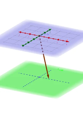
This example demonstrates mapping diagrams for quartic equations, visually illustrating the relationship between roots and function values in the complex plane. It involves core mathematical concepts such as complex numbers, symmetry, real numbers, geometric mean, and parametric curves. Key GeoGebra commands and objects used include ComplexRoot, Sequence, Zip, Vector, CurveCartesian, PointIn, Intersect, Circle, Center, Point, Locus, and Radius. Suitable for high school and advanced learners to understand complex function behavior and root distribution.
GeoGebra Commands & Parameters
ComplexRoot(f) → r_1, r_2, r_3, r_4Sequence((δ * (cos(t) + (sin(t) * ί))) + real(z_#) + (imaginary(z_#) * ί), t, -3.14159, π, (2 * π / m)) → z_*Zip(f3_C[r, p, q, z], z, z_*) → fz_*Sequence((x(Element[fz_*, k]), y(Element[fz_*, k]), height_{image}), k, 1, m) → fpoint_*Vector(z_#, f_{(z#).}) → wCurveCartesian(t, 0, height_{image}, t, -5, 5) → XhCurveCartesian(0, t, height_{image}, t, -5, 5) → YhPointIn(C_{image}) → LSequence(Vector[Element[z_*, j], Element[fpoint_*, j]], j, 1, m) → fvec_*Intersect(f, xAxis) → A, B, C, DZip(Vector[(x(z), y(z), 0), (0, 0, height_{image})], z, roots) → rootsvecCircle(r_3, r_2, r_1) → cCenter(c) → O_rPoint(circle) → P_CLocus(F_D, P_C) → f_{circ}Radius(c) → δ_r
AI Drawing Prompt Reference
Create a mapping diagram for a quartic equation, illustrating the relationship between roots and function values in the complex plane. Start by plotting the complex roots, then generate parametric curves, followed by the corresponding points on the image, connect these points with vectors, draw the x-axis and y-axis, mark points on the image, draw three concentric circles with the center as the circle's center, and finally, plot the locus of these circles.
The prompt above was compiled from the original drawing commands and is for reference only.