
Mapping Diagrams: Complex Analysis-functions with lines or circles
Loading the math board and drawing, please wait…
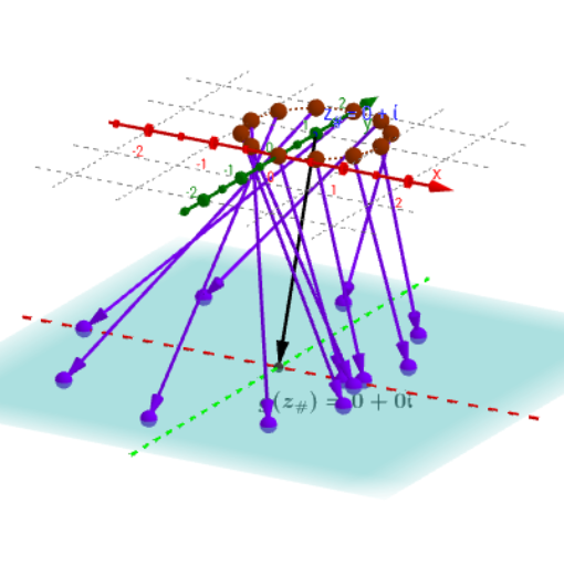
This example demonstrates how complex functions map input complex numbers to output lines or circles. Key math concepts include complex numbers, mapping, and geometric representation. Construction involves GeoGebra commands like Point, Sequence, Zip, Circle, Line, Vector, Locus. Suitable for high school students and beginners in complex analysis learning function properties and visualization.
GeoGebra Commands & Parameters
Point(Line_m) → A_lSequence(0, n) → MZip(((2 * π) * k / n), k, M) → t_*Zip(((m * (t - π)) * ί) + t - π + z_#, t, t_*) → z_lZip((δ * ℯ^((t * ί))) + z_#, t, t_*) → z_cCircle(z_#, δ) → circPoint(circ) → A_cIf(L1orC2 ≟ 2, z_c, z_l) → z_*Zip(h(z), z, z_*) → hz_*Zip((x(z), y(z), ht), z, hz_*) → hpt_*Line(O, ZY1) → YaxLine(O, ZX1) → XaxZip(Vector[A, B], A, z_*, B, hpt_*) → hvec1_*Vector(z_#, Gz1_#) → vecg_#Vector(z_#, Hz1_#) → vech_#If(L1orC2 ≟ 2, x(A_c) + (y(A_c) * ί), x(A_l) + (y(A_l) * ί)) → ATextfield(G) → InputBox1Textfield(H) → InputBox2Zip(g(z), z, z_*) → gz_*Zip((x(z), y(z), ht), z, gz_*) → gpt_*Zip(Vector[A, B], A, z_*, B, gpt_*) → gvec1_*Point(xAxis) → x_#Locus(gx_#, x_#) → grealLocus(hx_#, x_#) → hrealIf(L1orC2 ≟ 2, Locus[PtAG, A_c], Locus[PtAG, A_l]) → gLocIf(L1orC2 ≟ 2, Locus[PtAH, A_c], Locus[PtAH, A_l]) → hLoc