
Mapping Diagrams in Complex Analysis
Loading the math board and drawing, please wait…
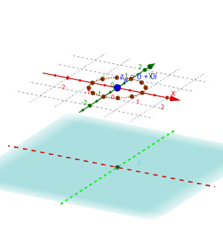
This example demonstrates mapping diagrams for complex functions and continuity. It involves core concepts like complex numbers, function mapping, and continuity. Constructed using GeoGebra commands and objects such as Textfield, Expand, Sequence, Zip, Circle, Line, Vector, Point, and Locus. Suitable for university mathematics students and learners of complex analysis.
GeoGebra Commands & Parameters
Textfield(G) → InputBox1Expand(Simplify[G(x + (y * ί), 0, x(a_#) + (y(a_#) * ί), 0, x(b_#) + (y(b_#) * ί), 0)]) → GzExpand(Simplify[H(x + (y * ί), 0, x(a_#) + (y(a_#) * ί), 0, x(b_#) + (y(b_#) * ί), 0, x(c_#) + (y(c_#) * ί), 0, x(d_#) + (y(d_#) * ί), 0)]) → HzTextfield(H) → InputBox2Sequence(0, m) → MZip(((2 * π) * k / m), k, M) → t_*Zip((δ * ℯ^((t * ί))) + z_#, t, t_*) → z_*Circle(z_#, δ) → cZip(Hr(x(z), y(z)) + (Hi(x(z), y(z)) * ί), z, z_*) → hz_*Zip(Gr(x(z), y(z)) + (Gi(x(z), y(z)) * ί), z, z_*) → gz_*Zip((x(z), y(z), ht), z, hz_*) → hpt_*Zip((x(z), y(z), ht), z, gz_*) → gpt_*Line(O, ZY1) → YaxLine(O, ZX1) → XaxZip(Vector[A, B], A, z_*, B, gpt_*) → gvec_*Zip(Vector[A, B], A, z_*, B, hpt_*) → hvec1_*Vector(z_#, Gz1_#) → vecg_#Vector(z_#, Hz1_#) → vech_#Point(c) → ALocus(PtAG, A) → gLocLocus(PtAH, A) → hLocCircle(Gz1_#, ε_g, xOyPlane) → cε_gCircle(Hz1_#, ε_h, xOyPlane) → cε_h